Topic: In this post, you will find an example of how to build and deploy a basic artificial
neural network scoring engine using
PL/SQL for recognizing handwritten digits. This post is intended for
learning purposes, in particular for Oracle practitioners who want a hands-on introduction to neural networks.
Introduction
Machine learning and
neural networks in particular, are currently hot topics in data processing. Many tools
and platform are now easily available to work and
experiment with neural networks and
deep learning (see also the links at the end of this post)
. Recognizing hand-written digits
, in particular using the
MNIST database by
Yann LeCun et al., is currently the "hello world" example for neural networks.
In this post, you will see how to build and deploy a simple neural network
scoring engine to recognize handwritten digits using
Oracle and PL/SQL. The final result is a short
PL/SQL package with an accuracy of about 98%. The neural network is built and trained using
TensorFlow and then transferred to Oracle for serving it.
One of the ideas that this post wants to illustrate is that scoring neural networks is much easier than training them: the operations required for
serving a trained network can be implemented relatively easily on many computing languages/environments. Discussions on these topics normally are centered around platforms for "Big Data" (see for example
Spark and
MLlib). I find
interesting to note that neural networks can also be successfully
applied to the RDBMS world. This can be useful as large quantities of valuable data are currently stored in
relational databases. In the case of Oracle, the implementation of a scoring engine is also made easier by the availability of a mature the PL/SQL environment with a package for
linear algebra: UTL_NLA.
Let's start from the end: how to deploy the PL/SQL package MNIST and recognize handwritten digits using Oracle
One short PL/SQL package and two tables is all you need to replay the following example (you can find the
details of the code on Github). The tables are:
- TENSORS_ARRAY: this table contains the numerical values for the vectors and matrices (tensors) that constitute the neural network. There is a total of 79510 floating point numbers encoded into four tensors using the data type UTL_NLA_ARRAY_FLT.
- TESTDATA_ARRAY: this table contains the test images. There are 10K images, each composed of 28x28 = 784 pixels. Image data is also encoded using the data type UTL_NLA_ARRAY_FLT.
The engine for scoring the example neural network is in a package called MNIST. It has a procedure called INIT that loads the components of the neural network from the table tensors_array into PL/SQL variables and a function called SCORE that takes an image as input and return a number, the predicted value of the digit.
Here is an example of its usage, where the first image in the table testdata_array is examined and correctly predicted to represent the number 7 (the image label agrees with the prediction by MNIST.SCORE):
SQL> exec mnist.init
PL/SQL procedure successfully completed.
SQL> select mnist.score(image_array), label from testdata_array where rownum=1;
MNIST.SCORE(IMAGE_ARRAY) LABEL
------------------------ ----------
7 7
Figure 1: This is a bitmap display of the test image used in the example. This confirms that the prediction of MNIST.SCORE is correct and indeed the image is a representation of the number 7 handwritten and encoded in a grid of 28x28 gray-scale pixels.
Processing all the test images is also a matter of a simple SQL command. In the example of Figure 2 it takes 2 minutes to process 10000 test images, that is about 12 ms per image on average. The
accuracy of the scoring function is about 98%. It is calculated as follows: out of 10000 images, 9787 are scored correctly according to the data labels. Note also that the set of test images is disjoint from the images used to train the neural network. Therefore we can expect that the MNIST package has an accuracy of about 98% for recognizing digits also when used on generic input (additional evaluations of the quality of the MNIST package as a classifier are beyond the scope of this post).
The full PL/SQL code and the datapump dump file with the relevant tables can be found on Github. In the following paragraphs, you can read how to build and train the neural network.
Figure 2: The accuracy of the PL/SQL scoring function MNIST.SCORE on the test set of 10K images is about 98%. Processing takes about 12 ms per image.
The neural network
The neural network used in this post is composed of three layers (see also Figure 3): one input layer, one hidden layer and one output layer. If this topic is new to you, I recommend to do some additional reading (see references) and in particular to read
Michael Nielsen's "
Neural Networks and Deep Learning" which provides an excellent introduction to the topic and a series of step-by-step examples on the problem of recognizing handwritten digits.
Figure 3: The artificial neural network used in this post is composed of three layers. The input layer has 784 neurons, one per pixel of the input image. A hidden layer of 100 neurons is added to improve the accuracy. The output layer has 10 neurons, one per each possible output value (that is digits from 0 to 9).
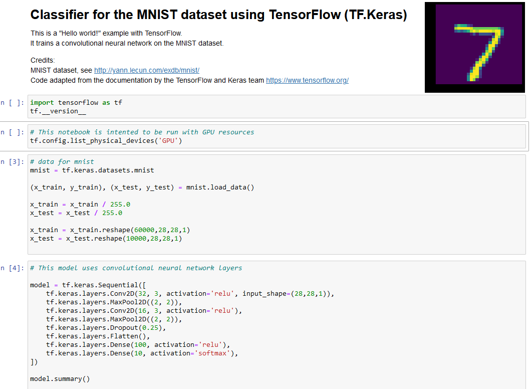
Get the training and test data, build and train the neural network using TensorFlow
Another important step for deploying neural networks is
training. For this you need
data, lots of it if possible. You also need an engine to do the necessary computation. Luckily there are many platforms available for working with neural networks, that that are free and relatively use to deploy (see references). In this post, you will see how to use Google's
TensorFlow and the Python environment.
TensorFlow comes with a
tutorial for recognizing handwritten digits in the
MNIST database. Included in the tutorial are training and test
data with
labels and also example
code.
You can find the code I used for training the neural network
on Github. Some highlights and code snippets are discussed in the following.
Importing the data: The example dataset that comes with TensorFlow provides 55000 images for training and 10000 images for testing. These originally come from the work of
Yann LeCun and coworkers. Having large amounts of high-quality data is very important to the success of the process. Moreover, the images come with
labels: the labels tell which number each image is intended to depict and provide a very important piece of information as the exercise is to do
supervised learning.
Defining the neural network: there are four tensors (vector and matrices in this case) in the network: W0, W1, b0 and b1. They are defined in the following snippet of code. To better understand their role and the key role that the cross entropy and the gradient descent optimizer play in training the network see the references, in particular "
Neural Networks and Deep Learning" and
TensorFlow tutorial.
Training the neural network: training proceeds with multiple steps of optimization. Training is performed using 55000 images with labels. It runs over 30000 iterations using "mini-batch" size of 100 images. At each step, the gradient descent algorithm computes an update of the weights and biases (W0, W1, bo and b1) with the goal of minimizing the loss function (cross_entropy). The relevant snippet of the code is:
Result: as a result, the trained network has the
accuracy of about 98% in recognizing the images in the test set. Note that the test set is composed of 10000 images and is disjoint from the set of images used for training (the training set contains 55000 images).
It is possible to get higher accuracy with more advanced neural network configurations (see references for details), but that is beyond the scope of this post.
Manually scoring the neural network, a Python example
The main result of the training operations is that the tensors (matrices and vectors in this case) that make the neural network are now populated with useful values. I believe that a good way to understand how all this works is to "run the network manually", that is run as an example of how to go from an image of a handwritten digit to the prediction of its value by the trained neural network. As a first step we
extract the values of the trained tensors in our model into
numpy arrays for later processing:
An example of
"manually" operating the network in Python is as follows:

W0_matrix, b0_array, W1_matrix and b1_array are the tensors that constitute the neural network after training, "testimage" is the input,
sigmoid() is used as activation function, "hidden_layer" represents the hidden layer of the network, "predicted" is the output layer and
softmax() is a function used to normalize the output as a probability distribution. At the end of the calculation, the array predicted[n] contains the prediction that the input image represents the digit "n". The function argmax() finds the value of "n" where
predicted[n] is maximized.
The code shown above predicts the value 7 for a test image. The prediction is confirmed as correct by the value of the label and can also be visually confirmed by the bitmap display of the test image (see Figure 1).
Move test data and neural network tensors to an Oracle database
The example in the previous paragraph on how to manually run a the scoring engine illustrates that
serving a neural network can be
straightforward, in some cases it is just a matter of performing some basic computations with matrices. This contrasts with the complexity of training neural network models, where often one needs a specialized engine, large quality of training data and in the more complex cases also specialized hardware, such as GPU cards.
The discussion of the previous paragraph has also prepared the terrain for the following development: that is
moving the neural network tensors and test data to Oracle and implement a serving engine there.
There are many ways to export Python's numpy arrays. One way is to
save them in a text format. Here you will see instead a method targeted to exporting directly into Oracle using cx_Oracle, the Python library to interact with Oracle. See also the notebook "
Oracle and Python with cx_Oracle" for additional examples and references on how to use cx_Oracle.
You can find the code
on Github, here are some relevant snippets:
-
Create the tables to host the tensor definition and test data:
SQL> create table tensors (name varchar2(20), val_id number, val binary_float, primary key(name, val_id));
SQL> create table testdata (image_id number, label number, val_id number, val binary_float, primary key(image_id, val_id));
- From Python, open a connection to Oracle:
import cx_Oracle
ora_conn = cx_Oracle.connect('mnist/mnist@ORCL')
cursor = ora_conn.cursor()
- Example of how to
transfer the matrix W0 into the Oracle table "tensors"
i=0
sql="insert into tensors values ('W0', :val_id, :val)"
for column in W0_matrix:
array_values = []
for element in column:
array_values.append((i, float(element)))
i += 1
cursor.executemany(sql, array_values)
ora_conn.commit()
Oracle's optimizations for linear algebra using UTL_NLA
From Oracle documentation: "The
UTL_NLA package exposes a subset of the
BLAS and LAPACK (Version 3.0) operations on vectors and matrices represented as VARRAYS". This is very useful for implementing the
calculations needed to serve the neural network of this post.
A snippet of the MNIST code to get the gist of this works in practice is reported below. The code performs the calculation v_Y0 = v_Y0 + g_W0_matrix * p_testimage_array, there g_W0_matrix is a
784x100 matrix, p_testimage_array is a vector of 784 elements (encoding the 28x28 images) and v_Y0 is a vector of 100 elements.
utl_nla.blas_gemv(
trans => 'N',
m => 100,
n => 784,
alpha => 1.0,
a => g_W0_matrix,
lda => 100,
x => p_testimage_array,
incx => 1,
beta => 1.0,
y => v_Y0,
incy => 1,
pack => 'C'
);
In order to use UTL_NLA the tensors that make the neural network and the test images need to be stored in varrays of binary_float, or rather be declared of data type UTL_NLA_ARRAY.
For this reason it is also convenient to post-process the tables "tensors" and "testdata" as follows:
SQL> create table testdata_array as
select a.image_id, a.label,
cast(multiset(select val from testdata where image_id=a.image_id order by val_id) as utl_nla_array_flt) image_array
from (select distinct image_id, label from testdata) a order by image_id;
SQL> create table tensors_array as
select a.name, cast(multiset(select val from tensors where name=a.name order by val_id) as utl_nla_array_flt) tensor_vals
from (select distinct name from tensors) a;
Finally, you can export the tables for later use. In the
Github repository you can find a dump file obtained with the following command (run as Oracle):
The final step, which brings you back to the discussion in the paragraph "let's start from the end: how to test the PL/SQL package MNIST", is to create the PL/SQL package MNIST that loads the tensors and performs the operations needed to score the neural network, See the details of the
code on Github.
Conclusions and comments
This post describes an example of how to implement a
scoring engine for an artificial
neural network using the
Oracle RDBMS and PL/SQL. The discussion is about a simple implementation of the "hello world" example of neural networks: recognizing handwritten digits of the
MNIST database. The network is trained using
TensorFlow and later exported into Oracle. The final result is a short PL/SQL package which provides digit recognition with an accuracy of about
98%.
We can expect in the near future to find
increasing deployments of
neural networks close to data sources and data stores. The example in this post of how to implement a neural network
serving engine on an
Oracle database shows that this is not only possible but also
easy to implement.
Serving neural networks is much
simpler than training them. While training requires specialized software/platforms and domain knowledge and large amounts of training data, trained networks can be imported into target systems and executed there, in many cases requiring low usage of computing resources.
This post is intended as
learning material: a simple feed forward neural network has been used instead of the more performing
convolutional network (see references). Moreover, data movement from TensorFlow to Oracle and the implementation of the serving engine in
PL/SQL is a sort of a
hack in the present state and it is not intended for production usage.
The code accompanying this post is available on Github.
Notes on how to build the test environment
The main components and tools for testing the scripts in this post are:
the
Python environment (on Linux with Centos 7) installed using
Anaconda 4.1: Python 2.7, Jupyter Ipython notebook.
TensorFlow, version 0.9 (the latest as I write this), installed following the instructions at
https://www.tensorflow.org/versions/r0.9/get_started/os_setup.html
Oracle RDBMS running on Linux. The Oracle scripts have been tested on Oracle 11.2.0.4 and 12.1.0.2
References and acknowledgments
An excellent introduction to neural networks and an inspiration for this blog post is
Michael Nielsen's book "
Neural Networks and Deep Learning".
The code for neural network training used in this post is an extension of Google's
TensorFlow MNIST
tutorial.
See also:
tutorial on TensorFlow by Martin Gorner
Basic techniques for TensorFlow by Aaron Schumacher
Visualizing MNIST by Christopher Olah
Python Machine Learning by Sebastian Raschka
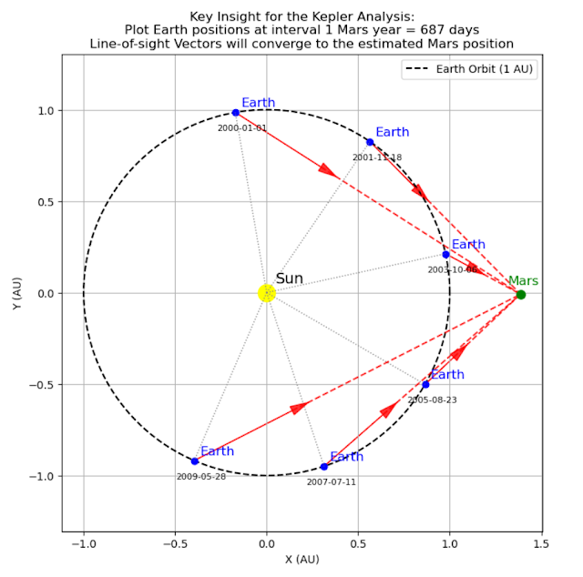
 Figure2: Demonstrate Kepler's First Law by fitting an elliptical model to confirm Mars’ orbit is an ellipse with the Sun at one focus. The fitted parameters match accepted values, notable eccentricity e ~ 0.09 and semi-major axis a ~ 1.52 AU.