Topic: This post describes a data pipeline for a machine learning task of interest in high energy physics: building a particle classifier to improve event selection at the particle detectors. The pipeline is built using tools from the "Big Data ecosystem", notably Apache Spark, BigDL and Analytics Zoo. The work is accompanied by
a set of notebooks with code and sample data.
The Physics use case
High Energy Physics (
HEP) is a
data-intensive domain: particle detectors and their sensors collect vast amounts of data. Data pipelines that move data from detectors to analysis engines are key to the experiments' success and operate at high throughput. For example, the amount of data flowing through the online systems at LHC experiments is currently of the order of
1 PB/s, with particle collision events happening every
25 ns. Most of the data thus collected has to be thrown away as it would be too costly to store the raw data. This is performed by fast data processing by a trigger system organized in multiple levels. The rate of data stored for later analysis is currently around 1-10 GB/sec.
Every improvement in the accuracy of the
event filtering system is welcome as it can provide large savings in terms of compute and storage resources needed for data analysis. The work "
Topology classification with deep learning to improve real-time event selection at the LHC" by Nguyen
et al. provides a promising solution to this problem by using
neural networks. The paper details how to build a classifier to used to improve the purity of data samples selected at trigger level, by distinguishing three different event topologies of interest ("W + jet", "QCD", "t tbar"). The classifier is intended to be used in the online filtering system to improve accuracy and in particular
reduce the number of
false positives compared to current systems, often implemented as complex rule-based systems.
The primary
goal of this work is to reproduce the classification performance results of
Nguyen et al., showing that the proposed
pipeline makes a more efficient usage of computing resources and/or provides a more
productive interface for the data scientist/physicists, along all the steps of the processing pipeline.
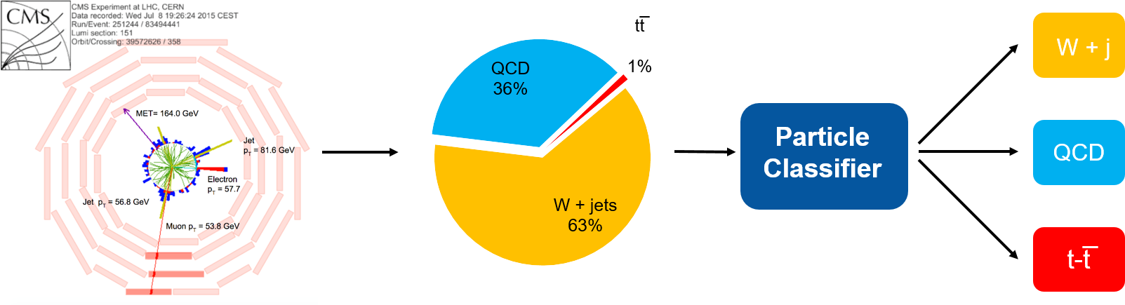
Figure 1: Event data collected from the particle detector (CMS experiment) contains different types of event topologies of interest. A particle classifier built with neural networks can be used as an event filter, improving state of the art in accuracy.
Data pipelines
Data pipelines are of paramount importance to make machine learning projects successful, by integrating multiple components and APIs used across the entire data processing chain. A good
data pipeline implementation can accelerate and improve the
productivity of the work around the core machine learning tasks. In particular, data pipelines are expected to provide solid tools for data processing, a task that ends up being one of the most
time-consuming for data scientists/physicists approaching data analysis problems.
Traditionally, HEP has developed
custom tools for data processing, which have been successfully used for decades. Recently, a large range of solutions for data processing and machine learning have become available from
open source communities. The maturity and adoption of such solutions continue to grow both in industry and academia. Using software from open source communities comes with several
advantages, including the
reduced cost of development and maintenance and the possibility of
sharing solutions and expertise with a large user and expert base.
In this work we build the
machine learning pipeline detailed in the paper on
topology classification with DL mentioned above, using tools from the "Big Data" ecosystem.
One of the key objectives for the machine learning data pipeline is to transform raw data into more valuable information used to train the ML/DL models.
Apache Spark provides the backbone of the pipeline, from the task of fetching data from the storage system to feature processing and feeding training data into a
DL engine (BigDL and Analytics Zoo are used in this work). The four steps of the pipeline we built are:
- Data Ingestion: where we read data from ROOT format and from the CERN-EOS storage system, into a Spark DataFrame and save the results as a table stored in Apache Parquet files
- Feature Engineering and Event Selection: where the Parquet files containing all the events details processed in Data Ingestion are filtered, and datasets with new features are produced
- Parameter Tuning: where the best set of hyperparameters for each model architecture are found by performing grid search
- Training: where the best models found in the previous step are trained on the entire dataset
Figure 2: This illustrates the data processing pipeline used for training the event topology classifier.
Data source
Data used for this work have been generated using software simulators to generate events and to calculate the detector response. The dataset is the result of a Monte Carlo event generation, where three different processes (categories) have been simulated: the inclusive production of a leptonically decaying W+/- boson, the pair production of a top-antitop pair (t, t_bar) and hadronic production of multijet events. Variables of low and high level are included in the dataset. See the paper on
topology classification with DL for details.
For this exercise, the generated training data amounts to 4.5 TB, for a total of
54 million events, divided in 3 classes:
"W + jet", "QCD", "t tbar" events. The generated training data is stored using the
ROOT format, as it is a very common format for HEP. Data are originally stored in the
CERN EOS storage system as it is the case for the majority of HEP data at CERN at present. The authors of the paper have kindly shared the training data for the purpose of this work. Each event of the dataset consists of a list of reconstructed particles. Each particle is associated with
features providing information on the particle cinematic (position and momentum) and on the type of particle.
Follow this link for additional details on the datasets and links to download data samples made available to reproduce this work.
Data ingestion
Data ingestion is the first step of the pipeline, where we read ROOT files from the
CERN EOS storage system into a Spark DataFrame. For this, we use a dedicated library able to
ingest ROOT data into Spark DataFrames: spark-root, an Apache Spark data source for the ROOT file format. It is based on a Java implementation of the
ROOT I/O libraries, which offers the ability to translate ROOT files into Spark DataFrames and RDDs. In order to access the files stored in the CERN EOS storage system from Spark applications, another library has been developed: the
Hadoop-XRootD connector. The Hadoop-XRootD connector is a Java library, it extends the HADOOP Filesystem and makes its capable of accessing files in EOS via the
XRootD protocol. This allows Spark to read directly from EOS. which is convenient for our use case as it avoids the need for copying data in HDFS or other storage compatible with Spark/Hadoop libraries.
At the end of the data ingestion step the result is that data, with the same structure as the original ROOT files, are made available as a Spark DataFrame on which we can perform event selection and feature engineering.
Event selection and feature engineering
In this step of the pipeline, we process the dataset by applying relevant filters, by computing derived features and by applying data normalization techniques.
The first part of the processing requires
domain-specific knowledge in HEP to simulate
trigger selection: this is emulated by requiring all the events to include one isolated electron or
muon with
transverse momentum (p_T) above a given threshold, p_T >= 23 GeV. All particle are then ranked in decreasing order of p_T. For each event, the isolated
lepton is the first entry of the list of particles. Together with the isolated lepton, the first 450 charged particles, the first 150 photons, and the first 200 neutral
hadrons have been considered, for a total of 801 particles with 19 features each. The result is, that each event passing the filter is associated to a matrix with shape
801 x 19. This defines the
Low Level Features (LLF) dataset.
Starting from the LLF, an additional set of
14 High Level Features (HLF) is computed. These additional features are motivated by known physics and data processing steps and will be of great help for improving the neural network model in later steps.
LLF and HLF datasets, computed as described above, are saved in Apache Parquet format: the amount of training data is reduced at this point from the original 4.4 TB of ROOT files to 950 GB of snappy-compressed Parquet files.
Additional processing steps are performed and include operations frequently found when preparing training data for classifiers, notably:
- Data undersampling. This is done to work around the class imbalance in the original training data. After this step, we have the same number of events per each of the three classes, that is 1.4 million events for each of the 3 classes.
- Data shuffling
- All the features present in the datasets are scaled to take values between 0 and 1 or normalized, as needed for the different classifiers.
- The datasets (for HLF and LLF features) are split in training and test datasets (80% and 20% respectively) and saved in two sets of Parquet files. Smaller datasets are also created as samples of the full train and test datasets, for development purposes,
Data are saved in snappy-compressed Parquet format at the end of this stage and amount to about 310 GB. The decrease in size from the previous step is mostly due to the undersampling step and the fact that the population on the 3 topology classes in the original training data used for this work are not balanced.
Code for this step: notebook for
data ingestion and for
feature preparation
Neural network models
We have tested three different neural network models, following the guiding
research paper:
1. The first and simplest model is the "
HLF Classifier". It is a fully connected feed-forward deep neural network taking as input the 14 high level features. The chosen architecture consists of three hidden layers with 50, 20, 10 nodes activated by Rectified Linear Units (ReLU). The output layer consists of 3 nodes, activated by the Softmax activation function.
2. The "
Particle Sequence Classifier" is trained using recursive layers, taking as input the 801 particles in the Low Level Features dataset. Prior to "feeding the particles" into a recurrent neural network, particles are ordered by decreasing distance from the isolated lepton (see the
original article for details).
Gated Recurrent Units (GRU) have been used to aggregate the input sequence of particles with a recurrent layer width of 50. The output of the GRU layer is fed into a fully connected layer with 3 Softmax-activated nodes.
3. The "
Inclusive Classifier" is the most complex of the 3 models tested. In this classifier, some domain knowledge is injected into the particle-sequence classifier. In order to do this, the architecture of the particle sequence classifier has been modified by concatenating the 14 High Level Features to the output of the GRU layer after a dropout layer. An additional dense layer of 25 nodes is introduced before the final output layer consisting of 3 nodes, activated by the Softmax activation function.
Figure 3: (left) Code snippet of the inclusive classifier model with Analytics zoo, using Keras-API. (right) Neural network model diagram from
Nguyen et al.
Parameter tuning
Hyperparameter tuning is a common step for improving machine learning pipelines. In this work, we have used Spark to speed up this step. Spark allows training multiple models with different parameters concurrently on a cluster, with the result of speeding up the hyperparameter tuning step. We used the Area Under the ROC curve as the performance metric to compare different classifiers. When performing a grid search each run is independent of the others, hence this process can be easily parallelized and scales very well.
For example, we tested the High Level Features classifier, a feed forward neural network, taking as input the 14 High Level Features. For this model, we tested changing the number of layers and units per layer, the activation function, the optimizer, etc. As an experiment, we ran grid search on the small dataset containing 100K events using a grid of ~200 hyper-parameters sets (models).
Hyperparameter tuning can similarly be repeated for all three classifiers described above. For the following work, we have decided to use the same models as the ones presented in the paper, as they were offering the best trade-off between performances and complexity.
To run grid search in parallel, we used Spark with
spark-sklearn and
Tensorflow/Keras wrapper for scikit_learn.
Code:
notebook with hyperparameter tuning
Figure 4: The hyperparameter tuning step consists of running multiple training jobs with the goal of finding an optimal set of parameters. Spark has been used to speed-up this step by running multiple Keras training jobs in parallel on a cluster.
Distributed training with Spark, BigDL and Analytics Zoo
There are many suitable software and platform solutions for deep learning training at present, and it is an exciting time in this respect with many paths to explore. However, choosing among them is not straightforward, as many products are available with different characteristics and optimizations for different areas of application.
For this work, we wanted to use a solution that easily integrates with the
Spark service at CERN, running on YARN/Hadoop cluster (more recently also running Spark on Kubernetes using cloud resources). GPUs and other HW accelerators are not yet available for Spark deployments at CERN, so we also wanted a solution that could scale on CPUs. Moreover, we wanted to use Python/PySpark and standard APIs for processing the neural network: notably Keras API in this case.
Those reasons combined with our ongoing collaboration with Intel in the context of
CERN openlab has led us to successfully test and use BigDL and Analytics Zoo for distributed model training in this work. BigDL and Analytics Zoo are
open source projects distributed under the Apache 2.0 license. They provide a distributed deep learning framework for Big Data platforms and are implemented as libraries on top of Apache Spark. They allow users to write large-scale deep learning applications as standard Spark programs, running on existing Spark clusters. Notably, they allow users to work with models defined with Keras and Tensorflow APIs.
BigDL provides data-parallelism to train models in a distributed fashion across a cluster using synchronous mini-batch Stochastic Gradient Descent. Data are automatically partitioned across Spark executors as an RDD of
Sample: an RDD of N-Dimensional array containing the input features and label. Distributed training is implemented as an iterative process, thus there will be multiple iterations over the same data. Reading data from disk multiple times is slow, for this reason, BigDL exploits the in-memory capabilities of Spark to cache the train RDD in the memory of each worker allowing faster access during the iterations (this also means that sufficient memory needs to be allocated for training large datasets).
More information on BigDL architecture can be found in the BigDL white paper.
Notebooks with the code used for training the DL models are:
Figure 5: Snippets of code illustrating key operations for deploying distributed model training in Spark using BigDL and Analytics Zoo.
The resulting classifiers show very good
performance figures for the three models tested, and reproduce the findings of the
original research paper. The fact that the HLF classifier performs well, despite its simplicity, can be justified by the fact that we are putting a considerable
physics knowledge into the the definition of the 14 high level features. This conclusion is further reinforced by additional tests, where we have built a topology classifier using a "
random decision forest" and a "gradient boosting" (
XGBoost) model, trained using the high level features dataset. In both cases we have obtained very good performance of the classifiers, just close to what has been achieved with the HLF classifier model.
In contrast, the fact that the
particle sequence classifier performs better than the HLF classifier is
remarkable, because we are not putting any
a priori knowledge into the particle sequence classifier: the model is taking just a list of particles as input. Further improvements are seen by combining the HLF with the particle sequence classifier. In some sense, the
GRU layer is identifying important features and physics quantities out of the training
data, rather than using knowledge injected via feature engineering.
Figure 6: (Right) ROC curve and AUC for the three models tested. Good results are obtained that are consistent with the findings in the
original research paper. (Left) Training and validation loss (categorical cross entropy) plotted as a function of iteration number for HLF classifier. Training convergence is obtained at around 50 epochs, depending on the model.
Figure 7: The
confusion matrix for the "Inclusive classifier" model after training. Note that the off-diagonal elements are below 5% and the diagonal elements are close to 95%.
Workload and performance
Two Spark clusters have been used to develop and run the workload, the first is a development/test cluster, the second is a production consisting of 52 nodes, with the following resources:
1800 vcores,
14 TB of RAM,
9 PB of storage. It is a shared general-purpose YARN/Hadoop cluster build on commodity hardware, installed with Linux (CentOS 7). Only a fraction of the resources of the cluster was used when executing the pipeline, moreover jobs of other nature were running on the system currently.
Data ingestion and
event filtering is a very
resource-demanding step of the pipeline. Processing the original data set of 4.4 TB took ~3 hours, using 50 executors with 8 cores each, for a total of
400 cores allocated to the Spark job.
Monitoring of the workload showed that the job was almost completely
CPU-bound. The large majority of the CPU cycles are spent executing Python code, that is outside of the Spark JVM. The fact that we chose to process the bulk of the training data using
Python UDF functions mapped on RDDs is the main cause of the use of such large amount of CPU resources, as this a well-known "performance gotcha" in current versions of Spark. Notably, many CPU cycles are "wasted" in data serialization and deserialization operations, going back and forth from JVM and Python, in the current implementation.
Additional work on
improving the performance of the event filtering has introduced the use of Spark SQL to implement some of the filters. Notably, we have made use of
Spark SQL Higher Order Functions, a specialized category of SQL functions, introduced in Spark from version 2.4.0, that allow to improve processing for nested data (arrays). For our workload this has introduced the benefit of running a significant fraction of the filtering operations fully inside the JVM, optimized by the Spark code for DataFrame operations. The result is that the data ingestion step, optimized with Spark SQL and higher order functions, runs in ~2 hours (was 3 hours in the implementation that uses only Python UDF).
Future work on the pipeline may further address the issue of reducing the time spent in serialization and deserialization when using Python UDF, for example, we might decide to re-write the critical parts of the ingestion code in
Scala. However, with the current training data size (4.4 TB), the performance of the data ingestion step, of just a couple of hours, is
acceptable.
Performance of
hyperparameter tuning with grid search: grid search runs multiple training jobs in parallel, therefore it is expected to
scale well when run in parallel, as it was the case in our work (see also the paragraph on hyperparameter tuning). This is confirmed by measurements, as shown in Figure 8, by adding executors, i.e. the number of models trained in parallel, the time required to scan all the parameters decreases, as expected.
Figure 8: Performance of the hyperparameter tuning with grid search shows near-linear scalability as expected by this embarrassingly parallel process.
Performance of
distributed training with BigDL and Analytics Zoo is also important for this exercise, as faster training time means improved productivity of the data scientist/physicists who will typically perform many experiments on the models and data. Figure 9 shows some preliminary results of the training
speed for the HLF classifier, tested on the development cluster, using batch size of 32 per worker. You can notice there very good
scalability behavior at the scale tested. Additional measurements, using 20 executors, with 6 cores each (for a total of 120 allocated cores), using batch size of 128 per worker, have shown training speed for the HLF classifier of the order of 100K rows/sec, sustained for the training of the full dataset. We have been able to train the model in less than
5 minutes, running for 12 epochs (each epoch processing 3.4 million training events). The batch size has an impact on the execution time and on the accuracy of the training. We found that a batch size of 128 for the HLF classifier is a good
compromise for speed, which a batch size of 32 is slower but gives slightly better results, for example for producing publication plots. Future work will address more thorough investigation of the performance and scalability of the training step.
Figure 9: Performance of the training step for the HLF classifier on the development cluster. Very good scalability has been found at this scale.
An important point to keep in mind when training models with BigDL, is that the RDDs containing the features and labels datasets need to be cached in the executors' JVM memory. This can be a significant amount of memory. Figure 10 shows the RDDs cached by Spark block manager when training the model "Inclusive classifier" using BigDL.
Figure 10: Datasets cached using Spark block manager when training the "Inclusive Classifier" model using BigDL. More than 200 GB of RAM are used across the Spark cluster to cache the training and test data.
The training dataset size and the model complexity of the HLF classifier are of relatively small scale, making the HLF classifier suitable for training also on desktop computers. However, the Particle sequence classifier and the Inclusive classifier have a much higher complexity and require processing hundreds of GB of training data. Figure 11 shows the amount of CPU consumed during the training of the Particle Sequence classifier using BigDL/Analytics-zoo on a Spark cluster, using 70 executor and training with a batch size of 32. Notably, Figure 11 illustrates the fact that the training has lasted for 9 hours and has utilized the equivalent of 200 CPUs for the whole duration of the training. The executor CPU measurement has been performed using Spark monitoring instrumentation feeding into an InfluxDB backed and visualized with Grafana, as
described in this post.
Figure 11: Measured aggregated CPU utilization of Spark executors during the training of the Particle Sequence classifier.
Conclusions, lessons learned and plans
We have successfully implemented the full
data pipeline for training a "topology classifier" for event filtering at LHC experiments, using
deep neural networks as detailed in an
original research paper using tools and platforms from the Big Data and machine learning ecosystem in the High Energy Physics domain.
Apache Spark has been used as the main engine for the pipeline, we have appreciated the flexibility and the ease of use of Spark's API in the Python environment.
The integration of PySpark with
Jupyter notebooks provides a user-friendly environment for data processing and exploration.
Additional key integrations with Spark have made this work possible, in particular, the
spark-root library allows Spark to read data in ROOT format and the
Hadoop-XRootD connector, which integrates Spark with CERN EOS storage system.
BigDL and
Analytics Zoo have allowed us to easily scale out training using familiar
Keras APIs and using the Spark clusters currently available at CERN.
We have identified areas for future performance improvements, notably in the data ingestion and filtering step where we chose to use Python functions on Spark RDDs for the current implementation.
Future work and plans include further exploration of the workload at scale, including running on cloud resources and investigating the use of HW accelerators for DL training. Another area we plan to explore in future work is to implement a streaming data pipeline with model inference, as the natural next step that follows this work.
Code for this work:
https://github.com/cerndb/SparkDLTrigger
Presentation at Spark Summit 2019:
Deep Learning on Apache Spark at CERN’s Large Hadron Collider with Intel Technologies
Acknowledgments
This work has been performed in the context of the Spark, Hadoop and Streaming services at CERN IT and has profited of the support and consultancy of the engineers in the service. The primary author of this work is Matteo Migliorini, who worked on it during his stay at CERN in 2018 under the supervision of Luca Canali. Additional credits go to Riccardo Castellotti, Viktor Khristenko and Maria Girone of CERN openlab, to Marco Zanetti of Padua University and to the authors of the research paper
Topology classification with deep learning to improve real-time event selection at the LHC", in particular to Maurizio Pierini and Thong Nguyen. Credits to the BigDL and Analytics Zoo team at Intel, in particular, many thanks to Jiao (Jennie) Wang and Sajan Govindan.