- Partition pruning
- Column projection
- Predicate/filter push-down
- Tools for investigating Parquet metadata
- Tools for measuring Spark metrics
Motivations: The combination of Spark and Parquet currently is a very popular foundation for building scalable analytics platforms. At least this is what we find in several projects at the CERN Hadoop and Spark service. In particular performance, scalability and ease of use are key elements of this solution that make it very appealing to our users. This also motivates the work described in this post on exploring the technology and in particular the performance characteristics of Spark workloads and internals of Parquet to better understand what happens under the hood, what works well and what are some of the current limitations.
The lab environment
This post is based on examples and short pieces of code that you should be able to try out in your test environments and experiment on why something works (or why it doesn't). I have used in this post a table from the schema of the TPCDS benchmark. The setup instructions for TPCDS on Spark can be found on Github at: "Spark SQL Performance Tests".
When testing the examples and measuring performance for this post, I have mostly used Spark on a YARN/Hadoop cluster of 12 nodes, however this is not a hard dependency: you can run your tests with similar results using local filesystem and/or Spark in local mode. I have run most of the examples using spark-shell, however the examples use Spark SQL so in most cases they will run unchanged on PySpark and/or on a notebook environment.
The labs discussed in this post have been tested using Spark version 2.2.0 (Release Candidate) and on Spark 2.1.1. Spark 2.2.0 depends on Parquet libraries version 1.8.2 (Spark 2.1.1 uses Parquet 1.8.1).
Test table in Parquet
The examples presented here use the TPCDS schema created with scale 1500 GB. Only one table is used in the examples, I have chosen to use the largest fact table: STORE_SALES. The table is partitioned and after the schema installation is physically located as a collection of Parquet files organized under a root directory.The total size is 185 GB in my lab environment. It adds up to 556 GB considering the 3-fold HDFS replication factor. This can be measured with:
$ hdfs dfs -du -h -s TPCDS/tpcds_1500/store_sales
185.3 G 556.0 G TPCDS/tpcds_1500/store_sales
The partitioning structure is visible by listing the content of the top-level directory. There are 1824 partitions in the test schema I used. Each partition is organized in a separate folder, the folder name contains the partition key. The files are compressed with snappy. The size of each individual file varies depending on the amount of data in the given partition. Here is an example of path and size of one of the files that constitute the store_sale table in my test schema:
Name: TPCDS/tpcds_1500/store_sales/ss_sold_date_sk=2452621/part-00077-57653b27-17f1-4069-85f2-7d7adf7ab7df.snappy.parquet
Bytes: 208004821
Spark and Parquet
Partitioning is a feature of many databases and data processing frameworks and it is key to make Spark jobs work at scale. Spark deals in a straightforward manner with partitioned tables in Parquet. The STORES_SALES from the TPCDS schema described in the previous paragraph is an example of how partitioning is implemented on a filesystem (HDFS in that case). Spark can read tables stored in Parquet and performs partition discovery with a straightforward API. This is an example of how to read the STORE_SALES table into a Spark DataFrame
val df = spark.read.
format("parquet").
load("TPCDS/tpcds_1500/store_sales")
This is an example of how to write a Spark DataFrame df into Parquet files preserving the partitioning (following the example of table STORE_SALES the partitioning key is ss_sold_date_sk):
df.write.
partitionBy("ss_sold_date_sk").
parquet("TPCDS/tpcds_1500/store_sales_copy")
Partition pruning
Let's start the exploration with something simple: partition pruning. This feature, common to most systems implementing partitioning, can speed up your workloads considerably by reducing the amount of I/O needed to process your query/data access code. The underlying idea behind partition pruning, at least in its simplest form for single-table access as in the example discussed here, is to read data only from a list of partitions, based on a filter on the partitioning key, skipping the rest. An example to illustrate the concept is query (2) (see below if you want to peek ahead). Before getting to that, however, I want to introduce a "baseline workload" with the goal of having a reference point for comparing the results of all the optimizations that we are going to test in this post.
1. Baseline workload: full scan of the table, no partition pruning
I have used spark-shell on a YARN cluster in my tests. You can also reproduce this in local mode (i.e. using --master local[*]) and/or use pyspark or a notebook to run the tests if you prefer. An example of how to start spark-shell (customize as relevant for your environment) is:
$ spark-shell --num-executors 12 --executor-cores 4 --executor-memory 4g
The next step is to use the Spark Dataframe API to lazily read the files from Parquet and register the resulting DataFrame as a temporary view in Spark.
spark.read.format("parquet").load("TPCDS/tpcds_1500/store_sales").createOrReplaceTempView("store_sales")
This Spark SQL command causes the full scan of all partitions of the table store_sales and we are going to use it as a "baseline workload" for the purposes of this post.
// query (1), this is a full scan of the table store_sales
spark.sql("select * from store_sales where ss_sales_price=-1.0").collect()
The query reads about 185 GB of data and 4.3 billion rows in my tests. You can find this type of performance metrics from the Spark Web UI (look for stage metrics: Input Size / Records), or with the tool sparkMeasure discussed later in this post. Here are the key metrics measured on a test of query (1):
- Total Time Across All Tasks: 59 min
- Locality Level Summary: Node local: 1675
- Input Size / Records: 185.3 GB / 4319943621
- Duration: 1.3 min

Note: at this stage, you can ignore the where clause "ss_sales_price = -1.0" in the test query. It is there so that an empty result set is returned by the query (no sales price is negative), rather than returning 185 GB of data and flooding the driver! What happens when executing query (1) is that Spark has to scan all the table partitions (files) from Parquet before applying the filter "ss_sales_price = -1.0" so this example is still a valid illustration of the baseline workload of table full scan. Later in this post, you will find more details about how and why this works in the discussion on predicate push down.
This is an example of a query where Spark SQL can use partition pruning. The query is similar to the baseline query (1) but with the notable change of an additional filter on the partition key. The query can be executed by reading only one partition of the STORE_SALES table.
// query (2), example of partition pruning
spark.sql("select * from store_sales where ss_sold_date_sk=2452621 and ss_sales_price=-1.0").collect()
- Total Time Across All Tasks: 6 s
- Locality Level Summary: Node local: 48
- Input Size / Records: 198.6 MB / 4502609
- Duration: 3 s

To recap, this section has shown two examples of reading with Spark a partitioned table stored in Parquet. The first example (query 1) is the baseline workload, performing a full scan of the entire table, the second example (query 2) shows the I/O reduction when a filter on the partitioning key allows Spark to use partition pruning. If partition pruning was not used by Spark the second query would also have to full scan the entire table.
Column projection
The idea behind this feature is simple: just read the data for columns that the query needs to process and skip the rest of the data. Column-oriented data formats like Parquet can implement this feature quite naturally. This contrasts with row-oriented data formats, typically used in relational databases and/or systems where optimizing for single row insert and updates are at a premium.
Column projection can provide an important reduction of the work needed to read the table and result in performance gains. The actual performance gain depends on the query, in particular on the fraction of the data/columns that need to be read to answer the business problem behind the query.
For example the table "store_sales" used for the example query (1) and (2) has 23 columns. For queries that don't need to retrieve the values of all the columns of the table, but rather a subset of the full schema, Spark and Parquet can optimize the I/O path and reduce the amount of data read from storage.
This command shows that "store_sales" has 23 columns and displays their names and data type:
spark.sql("desc store_sales").show(50)
+--------------------+------------+-------+
| col_name| data_type|comment|
+--------------------+------------+-------+
| ss_sold_time_sk| int| null|
| ss_item_sk| int| null|
| ss_customer_sk| int| null|
| ss_cdemo_sk| int| null|
| ss_hdemo_sk| int| null|
| ss_addr_sk| int| null|
| ss_store_sk| int| null|
| ss_promo_sk| int| null|
| ss_ticket_number| int| null|
| ss_quantity| int| null|
| ss_wholesale_cost|decimal(7,2)| null|
| ss_list_price|decimal(7,2)| null|
| ss_sales_price|decimal(7,2)| null|
| ss_ext_discount_amt|decimal(7,2)| null|
| ss_ext_sales_price|decimal(7,2)| null|
|ss_ext_wholesale_...|decimal(7,2)| null|
| ss_ext_list_price|decimal(7,2)| null|
| ss_ext_tax|decimal(7,2)| null|
| ss_coupon_amt|decimal(7,2)| null|
| ss_net_paid|decimal(7,2)| null|
| ss_net_paid_inc_tax|decimal(7,2)| null|
| ss_net_profit|decimal(7,2)| null|
| ss_sold_date_sk| int| null|
+--------------------+------------+-------+
The following example, query (3), is similar to the baseline query (1) discussed earlier, with the notable change that query (3) references 4 columns only: ss_sold_date_sk, ss_item_sk, ss_list_price with a filter on ss_sales_price. This allows Spark to reduce the amount of I/O performed compared to queries that need to read the entire table as query (1).
// query (3), an example of column pruning
spark.sql("select ss_sold_date_sk, ss_item_sk, ss_list_price from store_sales where ss_sales_price=-1.0").collect()
From the Web UI, after executing the query on a test system I find that it has read only 22.4 GB:
Compare this with the baseline query (1), which accessed 185 GB of data instead.
- Total Time Across All Tasks: 13 min
- Locality Level Summary: Node local: 1675
- Input Size / Records: 22.4 GB / 4319943621
- Duration: 18 s
The execution plan confirms that the query only needs to read data for the columns ss_sold_date_sk, ss_item_sk, ss_list_price:

Predicate push down
Predicate push down is another feature of Spark and Parquet that can improve query performance by reducing the amount of data read from Parquet files. Predicate push down works by evaluating filtering predicates in the query against metadata stored in the Parquet files. Parquet can optionally store statistics (in particular the minimum and maximum value for a column chunk) in the relevant metadata section of its files and can use that information to take decisions, for example, to skip reading chunks of data if the provided filter predicate value in the query is outside the range of values stored for a given column. This is a simplified explanation, there are many more details and exceptions that it does not catch, but it should give you a gist of what is happening under the hood. You will find more details later in this section and further in this post in the paragraph discussing Parquet internals.
An example where predicate push down can improve query performance
Here is an example where predicate push down is used to significantly improve the performance of a Spark query on Parquet.
// query (4), example of predicate push down
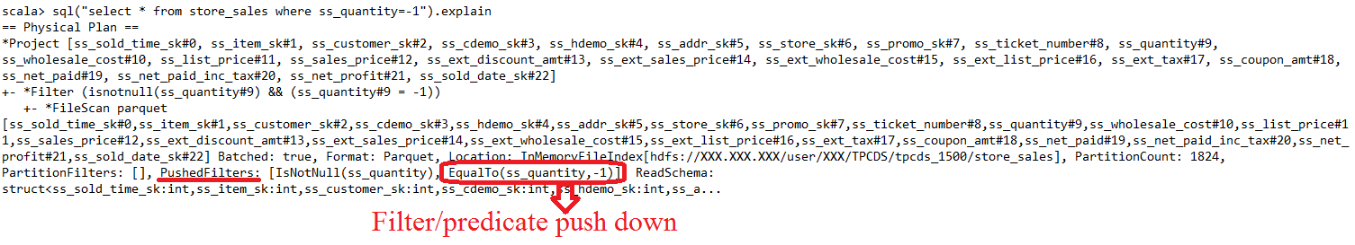
spark.sql("select * from store_sales where ss_quantity=-1").collect()
Query (4) is specially crafted with the filter predicate "where ss_quantity = -1". The predicate is never true in the STORE_SALES table (ss_quantity is a positive value). A powerful optimization can kick in in this case: Spark can push the filter to Parquet and Parquet can evaluate it against its metadata. As a consequence Spark and Parquet can skip performing I/O on data altogether with an important reduction in the workload and increase in performance. To be precise Spark/Parquet still need to access all the files that make the table to read the metadata, but this is orders of magnitude faster than reading the data. You can see that by comparing the execution metrics of query (4) with the baseline query (1):
- Total Time Across All Tasks: 1.0 min
- Locality Level Summary: Node local: 1675
- Input Size / Records: 16.2 MB / 0
- Duration: 3 s
The execution plan shows that the filter is indeed pushed down to Parquet:
There are exceptions when predicate push down cannot be used
This example brings us back to query(1):// query(1), baseline with full scan of store_sales
spark.sql("select * from store_sales where ss_sales_price=-1.0").collect()
Question: if you compare query (1) and query (4), you will find that they look similar, however, their performance is quite different. Why?
The reason is that predicate push down does not happen for all datatypes in Parquet, in particular with the current version of Spark+Parquet (that is Parquet version 1.8.2, for the tests reported here with Spark 2.2.0 RC) predicates on column of type DECIMAL are not pushed down, while INT (integer) values are pushed down (see also PARQUET-281). The reference query (1) has a filter on ss_sales_price of type decimal(7,2), while query (4) has a predicate on ss_quantity that is of type INT.
Note on the execution plan: Spark physical execution plan for query (1) reports that the predicate "ss_sales_price=-1.0" is actually pushed down similarly to what you can see for query (2), this can be misleading as Parquet is not actually able to push down this value. The performance metrics, elapsed time and amount of data read, confirm that the table is scanned fully in the case on query (1).
Another important point is that only predicates using certain operators can be pushed down as filters to Parquet. In the example of query (4) you can see a filter with an equality predicate being pushed down.
Other operators that can be pushed down are "<, <=, > , >=". More details on the datatypes and operators that Spark can push down as Parquet filters can be found in the source code. For more details follow the link to ParquetFilters.scala for a relevant piece of the source code.
An example where predicate push down kicks in but with minimal gains in performance
Here is another example that can be useful to understand some of the limitations around filter push down. What executing query (5) Spark can push down the predicate to Parquet but the end result is only a small reduction in data read and therefore a minimal impact on performance.// query (5), another example of predicate push down
// This time however with small gains in performance, due to data distribution and filter value
spark.sql("select * from store_sales where ss_ticket_number=348594569").collect()
The stats are:
- Total Time Across All Tasks: 50 min
- Locality Level Summary: Node local: 1675
- Input Size / Records: 173.7 GB / 4007845204
- Duration: 1.1 min
Execution plan:

It is useful to understand the different behavior between query (4) and query (5). The reason is with the data: the value used for the filter "ss_ticket_number=348594569" has been cherry picked to be in inside the range between minimum and maximum for ss_ticket_number for most of the table partitions. To be more accurate the granularity at which Parquet stores metadata that can be used for predicate push down is called "row group" and is a subset of Parquet files. More on this in the section on Parquet internals and diagnostic tools.
Due to the nature of data and the value of the filter predicate, Parquet finds that the filter value is in the range of minimum-to-maximum value for most of the row groups. Therefore Parquet libraries end up reading the vast majority of the table in this example. For some partitions, predicate pushing kicks in and the actual amount of data read is a bit lower that the full table scan value in this example: 173 GB in query (5) vs. 185 GB in query (1).
The main takeaway from this example is that filter push down does not guarantee performance improvements in all cases, the actual gains in I/O reduction due to predicate push down depend on data distribution and on predicate values.
Comments:
You can also expect that as Parquet matures more functionality will be added to predicate pushing. A notable example of this trend in PARQUET-384 "Add Dictionary Based Filtering to Filter2 API", an improvement pushed to Parquet 1.9.0.
Parquet file push down is enabled by default in Spark, if you want to further experiment with it you can also use the following parameter to turn the feature <on|off>: spark.sql.parquet.filterPushdown=<true|false>
Drill down into Parquet metadata with diagnostic tools
The discussion on predicate push down in the previous section has touched on some important facts about Parquet internals. At this stage you may want to explore the internals of Parquet files and their metadata structure to further understand the performance of your the queries. One good resource for that is the documentation at https://parquet.apache.org/documentation/latest
Also the Parquet source code has many additional details in the form of comments to the code. See for example: ParquetOutputFormat.java
Some of the main points about Parquet internals that I want to highlight are:
- Hierarchically, a Parquet file consists of one or more "row groups". A row group contains data grouped ion "column chunks", one per column. Column chunks are structured in pages. Each column chunk contains one or more pages.
- Parquet files have several metadata structures, containing among others the schema, the list of columns and details about the data stored there, such as name and datatype of the columns, their size, number of records and basic statistics as minimum and maximum value (for datatypes where support for this is available, as discussed in the previous section).
- Parquet can use compression and encoding. The user can choose the compression algorithm used, if any. By default Spark uses snappy.
- Parquet can store complex data types and support nested structures. This is quite a powerful feature and it goes beyond the simple examples presented in this post.
Parquet-tools:
Parquet-tools is part of the main Apache Parquet repository, you can download it from https://github.com/apache/parquet-mr/releases
The tests described here are based on Parquet version 1.8.2, released in January 2017. Note: Parquet version 1.9.0 is also out since October 2016, but it is not used by Spark, at least up to Spark version 2.2.0.
Tip: you can build and package the jar for parquet-tools with:
cd parquet-mr-apache-parquet-1.8.2/parquet-tools
mvn package
You can use parquet tools to examine the metadata of a Parquet file on HDFS using: "hadoop jar <path_to_jar> meta <path_to_Parquet_file>". Other commands available with parquet-tools, besides "meta" include: cat, head, schema, meta, dump, just run parquet-tools with -h option to see the syntax.
$ echo "read metadata from a Parquet file in HDFS"
$ hadoop jar parquet-mr-apache-parquet-1.8.2/parquet-tools/target/parquet-tools-1.8.2.jar meta TPCDS/tpcds_1500/store_sales/ss_sold_date_sk=2452621/part-00077-57653b27-17f1-4069-85f2-7d7adf7ab7df.snappy.parquet
The output lists several details of the file metadata:
file path, parquet version used to write the file (1.8.2 in this case), additional info (Spark Row Metadata in this case):
file path, parquet version used to write the file (1.8.2 in this case), additional info (Spark Row Metadata in this case):
file: hdfs://XXX.XXX.XXX/user/YYY/TPCDS/tpcds_1500/store_sales/ss_sold_date_sk=2452621/part-00077-57653b27-17f1-4069-85f2-7d7adf7ab7df.snappy.parquet
creator: parquet-mr version 1.8.2 (build c6522788629e590a53eb79874b95f6c3ff11f16c)
extra: org.apache.spark.sql.parquet.row.metadata = {"type":"struct","fields":[{"name":"ss_sold_time_sk","type":"integer","nullable":true,"metadata":{}},{"name":"ss_item_sk","type":"integer","nullable":true,"metadata":{}},
...omitted in the interest of space...
{"name":"ss_net_profit","type":"decimal(7,2)","nullable":true,"metadata":{}}]}
Additionally metadata about the schema:
file schema: spark_schema
--------------------------------------------------------------
ss_sold_time_sk: OPTIONAL INT32 R:0 D:1
ss_item_sk: OPTIONAL INT32 R:0 D:1
ss_customer_sk: OPTIONAL INT32 R:0 D:1
ss_cdemo_sk: OPTIONAL INT32 R:0 D:1
ss_hdemo_sk: OPTIONAL INT32 R:0 D:1
ss_addr_sk: OPTIONAL INT32 R:0 D:1
ss_store_sk: OPTIONAL INT32 R:0 D:1
ss_promo_sk: OPTIONAL INT32 R:0 D:1
ss_ticket_number: OPTIONAL INT32 R:0 D:1
ss_quantity: OPTIONAL INT32 R:0 D:1
ss_wholesale_cost: OPTIONAL INT32 O:DECIMAL R:0 D:1
ss_list_price: OPTIONAL INT32 O:DECIMAL R:0 D:1
ss_sales_price: OPTIONAL INT32 O:DECIMAL R:0 D:1
ss_ext_discount_amt: OPTIONAL INT32 O:DECIMAL R:0 D:1
ss_ext_sales_price: OPTIONAL INT32 O:DECIMAL R:0 D:1
ss_ext_wholesale_cost: OPTIONAL INT32 O:DECIMAL R:0 D:1
ss_ext_list_price: OPTIONAL INT32 O:DECIMAL R:0 D:1
ss_ext_tax: OPTIONAL INT32 O:DECIMAL R:0 D:1
ss_coupon_amt: OPTIONAL INT32 O:DECIMAL R:0 D:1
ss_net_paid: OPTIONAL INT32 O:DECIMAL R:0 D:1
ss_net_paid_inc_tax: OPTIONAL INT32 O:DECIMAL R:0 D:1
ss_net_profit: OPTIONAL INT32 O:DECIMAL R:0 D:1
Metadata about the row groups:

Note: If you want to investigate further, you can also dump information down to the page level using the command: parquet-tools command "dump --disable-data" on the Parquet file of interest.
file schema: spark_schema
--------------------------------------------------------------
ss_sold_time_sk: OPTIONAL INT32 R:0 D:1
ss_item_sk: OPTIONAL INT32 R:0 D:1
ss_customer_sk: OPTIONAL INT32 R:0 D:1
ss_cdemo_sk: OPTIONAL INT32 R:0 D:1
ss_hdemo_sk: OPTIONAL INT32 R:0 D:1
ss_addr_sk: OPTIONAL INT32 R:0 D:1
ss_store_sk: OPTIONAL INT32 R:0 D:1
ss_promo_sk: OPTIONAL INT32 R:0 D:1
ss_ticket_number: OPTIONAL INT32 R:0 D:1
ss_quantity: OPTIONAL INT32 R:0 D:1
ss_wholesale_cost: OPTIONAL INT32 O:DECIMAL R:0 D:1
ss_list_price: OPTIONAL INT32 O:DECIMAL R:0 D:1
ss_sales_price: OPTIONAL INT32 O:DECIMAL R:0 D:1
ss_ext_discount_amt: OPTIONAL INT32 O:DECIMAL R:0 D:1
ss_ext_sales_price: OPTIONAL INT32 O:DECIMAL R:0 D:1
ss_ext_wholesale_cost: OPTIONAL INT32 O:DECIMAL R:0 D:1
ss_ext_list_price: OPTIONAL INT32 O:DECIMAL R:0 D:1
ss_ext_tax: OPTIONAL INT32 O:DECIMAL R:0 D:1
ss_coupon_amt: OPTIONAL INT32 O:DECIMAL R:0 D:1
ss_net_paid: OPTIONAL INT32 O:DECIMAL R:0 D:1
ss_net_paid_inc_tax: OPTIONAL INT32 O:DECIMAL R:0 D:1
ss_net_profit: OPTIONAL INT32 O:DECIMAL R:0 D:1
Metadata about the row groups:
Note: If you want to investigate further, you can also dump information down to the page level using the command: parquet-tools command "dump --disable-data" on the Parquet file of interest.
Parquet_reader
Parquet_reader This is another utility that can help you navigate the internals and metadata of Parquet files. In particular parquet-cpp displays the statistics associated with Parquet columns and is useful to understand predicate push down.
Parquet_reader is a utility distributed with the Parquet-cpp project.
You can download it from https://github.com/apache/parquet-cpp/releases
The tests reported here have been run using version 1.1.0 released in May 2017.
Tips: You can build the project with: "cmake ." followed by "make". After that you can find the utility parquet_reader in the folder build/latest.
This is an example of how to use parquet_reader to browse file metadata. The tool works on filesystem data, so I have copied the parquet file from HDFS to local filesystem before running this:
./parquet_reader --only-metadata part-00077-57653b27-17f1-4069-85f2-7d7adf7ab7df.snappy.parquet
File metadata: similarly to the case of parquet-tools you can find the list of columns and their data types. Note however that DECIMAL columns are not identified.
File Name: part-00077-57653b27-17f1-4069-85f2-7d7adf7ab7df.snappy.parquet
Created By: parquet-mr version 1.8.2 (build c6522788629e590a53eb79874b95f6c3ff11f16c)
Total rows: 2840100
Number of RowGroups: 2
Number of Real Columns: 22
Number of Columns: 22
Number of Selected Columns: 22
Column 0: ss_sold_time_sk (INT32)
Column 1: ss_item_sk (INT32)
Column 2: ss_customer_sk (INT32)
Column 3: ss_cdemo_sk (INT32)
Column 4: ss_hdemo_sk (INT32)
Column 5: ss_addr_sk (INT32)
Column 6: ss_store_sk (INT32)
Column 7: ss_promo_sk (INT32)
Column 8: ss_ticket_number (INT32)
Column 9: ss_quantity (INT32)
Column 10: ss_wholesale_cost (INT32)
Column 11: ss_list_price (INT32)
Column 12: ss_sales_price (INT32)
Column 13: ss_ext_discount_amt (INT32)
Column 14: ss_ext_sales_price (INT32)
Column 15: ss_ext_wholesale_cost (INT32)
Column 16: ss_ext_list_price (INT32)
Column 17: ss_ext_tax (INT32)
Column 18: ss_coupon_amt (INT32)
Column 19: ss_net_paid (INT32)
Column 20: ss_net_paid_inc_tax (INT32)
Column 21: ss_net_profit (INT32)
--- Row Group 0 ---
--- Total Bytes 154947976 ---
Rows: 2840100---
Column chunk metadata: similarly to the case of parquet-tools you can find details on the number of rows and the compressed/uncompressed size. In addition parquet_reader shows the statistics of Minimum and Maximum values. Also the number of null values are reported, while distinct values appears to be 0 (not populated).
Column 0
, Values: 2840100, Null Values: 66393, Distinct Values: 0
Max: 75599, Min: 28800
Compression: SNAPPY, Encodings: RLE PLAIN_DICTIONARY BIT_PACKED
Uncompressed Size: 5886233, Compressed Size: 2419027
Column 1
, Values: 2840100, Null Values: 0, Distinct Values: 0
Max: 32000, Min: 1
Compression: SNAPPY, Encodings: RLE PLAIN_DICTIONARY BIT_PACKED
Uncompressed Size: 5040503, Compressed Size: 5040853
Column 2
, Values: 2840100, Null Values: 66684, Distinct Values: 0
Max: 4599961, Min: 15
Compression: SNAPPY, Encodings: RLE PLAIN_DICTIONARY BIT_PACKED
Uncompressed Size: 7168827, Compressed Size: 4200678
...
Notably, there are no statistics for columns of type DECIMAL. This has implications for filter push down, as discussed earlier in this post. See for example:
...
Column 10
, Values: 2840100 Statistics Not Set
Compression: SNAPPY, Encodings: RLE PLAIN_DICTIONARY BIT_PACKED
Uncompressed Size: 5113188, Compressed Size: 5036313
Column 11
, Values: 2840100 Statistics Not Set
Compression: SNAPPY, Encodings: RLE PLAIN_DICTIONARY BIT_PACKED
Uncompressed Size: 5500119, Compressed Size: 5422519
...
sparkMeasure for measuring Spark metrics
Spark performance metrics are exposed via the WebUI and REST API. In addition to that a small custom-developed tool to measure Spark Task Metrics and SQL metrics is sparkMeasure. I have described it in the blog post "On Measuring Apache Spark Workload Metrics for Performance Troubleshooting".
To use sparkMeasure, download the jar or point to its coordinates on Maven Central as in this example: bin/spark-shell --packages ch.cern.sparkmeasure:spark-measure_2.11:0.11
This is an example of how to measure metrics for Spark SQL using sparkMeasure:
val stageMetrics = ch.cern.sparkmeasure.StageMetrics(spark)
stageMetrics.runAndMeasure(spark.sql("select * from store_sales where ss_sales_price=-1").collect())
Spark Context default degree of parallelism = 48
Aggregated Spark stage metrics:
numStages => 1
sum(numTasks) => 1675
elapsedTime => 75684 (1.3 min)
sum(stageDuration) => 75684 (1.3 min)
sum(executorRunTime) => 3525951 (59 min)
sum(executorCpuTime) => 1006093 (17 min)
sum(executorDeserializeTime) => 4410 (4 s)
sum(executorDeserializeCpuTime) => 2106 (2 s)
sum(resultSerializationTime) => 69 (69 ms)
sum(jvmGCTime) => 811933 (14 min)
sum(shuffleFetchWaitTime) => 0 (0 ms)
sum(shuffleWriteTime) => 0 (0 ms)
max(resultSize) => 2346124 (2.0 MB)
sum(numUpdatedBlockStatuses) => 48
sum(diskBytesSpilled) => 0 (0 Bytes)
sum(memoryBytesSpilled) => 0 (0 Bytes)
max(peakExecutionMemory) => 0
sum(recordsRead) => 4319943621
sum(bytesRead) => 198992404103 (185.0 GB)
sum(recordsWritten) => 0
sum(bytesWritten) => 0 (0 Bytes)
sum(shuffleTotalBytesRead) => 0 (0 Bytes)
sum(shuffleTotalBlocksFetched) => 0
sum(shuffleLocalBlocksFetched) => 0
sum(shuffleRemoteBlocksFetched) => 0
sum(shuffleBytesWritten) => 0 (0 Bytes)
sum(shuffleRecordsWritten) => 0
scala> stageMetrics.printAccumulables
Aggregated Spark accumulables of type internal.metric. Sum of values grouped by metric name
Name => sum(value) [group by name]
executorCpuTime => 1006093 (17 min)
executorDeserializeCpuTime => 2106 (2 s)
executorDeserializeTime => 4410 (4 s)
executorRunTime => 3525951 (59 min)
input.bytesRead => 198992404103 (185.0 GB)
input.recordsRead => 4319943621
jvmGCTime => 811933 (14 min)
resultSerializationTime => 69 (69 ms)
resultSize => 2346124 (2.0 MB)
SQL Metrics and other non-internal metrics. Values grouped per accumulatorId and metric name.
Accid, Name => max(value) [group by accId, name]
256, number of output rows => 4319943621
259, scan time total => 3327453 (55 min)
260, duration total => 3522020 (59 min)
Conclusions
Spark and Parquet are currently the core technology for many analytics platforms. This post covers some of the basic features and workloads by example that highlight how Spark + Parquet can be useful when handling large partitioned tables, a typical use case for data warehousing and analytics. In particular partition discovery, partition pruning, data compression, column projection and filter push down are covered in this post. In addition this post shows some examples of diagnostic tools for exploring Parquet metadata (parquet-tools, parquet_reader) and tools to measure Spark workloads (Spark WebUI and a custom tool sparkMeasure). This only scratches the surface of what is there to explore and experiment with Spark and Parquet, I hope the readers will have much more fun with their own investigations.
References
Spark programming guide: https://spark.apache.org/docs/latest/sql-programming-guide.html
Parquet documentation https://parquet.apache.org/
Parquet file format description: https://github.com/apache/parquet-format/blob/master/src/main/thrift/parquet.thrift
Spark + Parquet In Depth, Spark Summit East talk: https://www.youtube.com/watch?v=_0Wpwj_gvzg Parquet file format description: https://github.com/apache/parquet-format/blob/master/src/main/thrift/parquet.thrift
Recent work on and around Parquet is can be followed at https://twitter.com/ApacheParquet
For the lab setup with the TPCDS schema for Spark see https://github.com/databricks/spark-sql-perf and also https://github.com/gregrahn/tpcds-kit
Acknowledgements
This work has been developed in the context of the CERN Hadoop and Spark service and is built thanks to the contributions of several of my colleagues there.
Bonus material
I have some spill over material for this post that I add here in the form of a few additional questions related to reading Parquet with Spark. The idea is that that you may be interested to use these questions as a learning exercise. It would take too long to discuss the questions and answers in details, for the moment I have only added some hints.
Question 1: At first though a simple implementation of the baseline workload for table scan would be to just count the elements in Parquet table (DataFrame in Spark). I mean something like spark.sql("select count(*) from store_sales").collect(). It appears a simpler than the SQL proposed in query (1) above, moreover you may be used to run a count(*) query in other database systems to cause a full scan of the table. Can you explain what is wrong with using count() to measure the performance or reading from Parquet files?
Question 2: Why does the partitioning column "ss_sold_date_sk" of the table store_sales does not appear in the Parquet metadata dumps performed with parquet-tools and parquet_reader?
Question 3: The table store_sales has 1824 partitions in my test sample. However, after reading it into Spark the Spark DataFrame has only 1675 partitions in my tests (note the number of partitions in a Dataframe df can be found with the command "df.rdd.partitions.size"). You should also find a similar difference in your test systems. Can you explain the difference between the number of partition in Parquet and Spark?
Can you describe the rules for populating Spark partitions when reading Parquet files?
Question 4: What happens if you write a Spark DataFrame to Parquet without specifying the partitionBy clause. Will the resulting table be partitioned?
Question 5: How can you configure the size of the row group in parquet? Experiment with different sizes and see the results by dumping the metadata.
Hints to the questions:
Hint 1: Look at Parquet metadata and where to find the information on row count.
Hint 2: The partitioning column is rather picked up by looking at the directory structure where doing partition discovery.
Hint 3: Experiment also with setting spark.sql.files.maxPartitionBytes (defaults to 128 MB, which is also the default for Parquet block size)
Hint 4: Examine the resulting directory structure on the filesystem.
Hint 5: Experiment with changing the Parquet block size using: sc.hadoopConfiguration.setInt("parquet.block.size",256*1024*1024)