Thursday, February 23, 2023

Introduction to Spark APIs for Data Processing

Introduction to Apache Spark APIs for Data Processing

This is a self-paced and open introduction course to Apache Spark. Theory and demos cover the main Spark APIs: DataFrame API, Spark SQL, Streaming, Machine Learning. You will also learn how to deploy Spark on CERN computing resources, notably using the CERN SWAN service. Most tutorials and exercises are in Python and run on Jupyter notebooks.

The main course website can be found at https://sparktraining.web.cern.ch/

Apache Spark is a popular engine for data processing at scale. Spark provides an expressive API and a scalable engine that integrates very well with the Hadoop ecosystem as well as with Cloud resources. Spark is currently used by several projects at CERN, notably by IT monitoring, by the security team, by the BE NXCALS project, by teams in ATLAS and CMS. Moreover, Spark is integrated with the CERN Hadoop service, the CERN Cloud service, and the CERN SWAN web notebooks service.


Accompanying notebooks

·       Get the notebooks from:

o   https://github.com/cerndb/SparkTraining

o   https://gitlab.cern.ch/db/SparkTraining

·     How to run the notebooks:

o   CERN SWAN (recommended option):

See also the SWAN gallery and the video:

o   Colab , Binder

o   Your local/private Jupyter notebook


Course lectures and tutorials

·       Introduction and objectives: slides and video


·       Session 1: Apache Spark fundamentals

o   Lecture “Spark architecture and intro to DataFrames”: slides and video

Graphical user interface, diagram

Description automatically generated

o   Notebooks:

o   Tutorial on DataFrames with exercisesvideo Icon

Description automatically generated

o   Solutions to the exercises

·       Session 2: Working with Spark DataFrames and SQL

o   Lecture “Introduction to Spark SQL”: slides and video


o   Notebooks:

o   Tutorial on Spark SQLvideo Icon

Description automatically generated

o   Exercises on Spark SQL

o   Solutions to the exercises

·       Session 3: Building on top of the DataFrame API

o   Lecture “Spark as a Data Platform”: slides and video


o   Lecture “Spark Streaming”: slides and video


o   Lecture “Spark and Machine Learning”: slides and video


o   Notebooks:

o   Tutorial on Spark Streamingvideo Icon

Description automatically generated

o   Tutorial on Spark Machine Learning – regression taskvideo Icon

Description automatically generated

o   Tutorial on Spark Machine Learning – classification task with the Higgs dataset

o   Demo of the Spark JDBC data source how to read Oracle tables from Spark

o   Note on Spark and Parquet format

·       Session 4: How to scale out Spark jobs

o   Lecture “Running Spark on CERN resources”: slides and video


o   Notebooks:

o   Demo on using SWAN with Spark on Hadoopvideo Icon

Description automatically generated

o   Demo of Spark processing Physics data using CERN private Cloud resourcesvideo Icon

Description automatically generated

o   Example notebook for the NXCALS project


·       Bonus material:

o   How to monitor Spark execution: slides and video Icon

Description automatically generated

o   Spark as a library, examples of how to use Spark in Scala and Python programs: code and video Icon

Description automatically generated

o   Next steps: reading material and links, miscellaneous Spark notes


·       Read and watch at your pace:

o   Download the course material for offline use:
 slides.zip, github_repo.zip, videos.zip

o   Watch the videos on YouTube Logo, icon

Description automatically generated


Acknowledgements and feedback

Author and contact for feedback and questions: Luca Canali - Luca.Canali@cern.ch

CERN-IT Spark and data analytics services

Former contributors: Riccardo Castellotti, Prasanth Kothuri

Many thanks to CERN Technical Training for their collaboration and support


License: CC BY-SA 4.0

Published in November 2022

Reposted from https://sparktraining.web.cern.ch/


Monday, May 23, 2022

Making histograms with Apache Spark and other SQL engines

Topic: This post will show you how to generate histograms using Apache Spark. You will find examples using the Spark DataFrame API and with a custom helper package, SparkHistogram. Additional examples will extend the work to histogram generation for several other databases and SQL engines.  

Disambiguation: we refer here to computing histograms for data analysis, rather than histograms of table columns or statistics used by cost- based optimizers.


Why histograms with Apache Spark?

Histograms are common tools for data analysis and are a key element in most High Energy Physics analyses. See also the post Can High Energy Physics Analysis Profit from Apache Spark APIs?

The advantage of generating histograms using Apache Spark, or other distributed data engines, is that the computation can be run at scale, with higher bandwidth to the data. This is useful if you have large datasets, for example, datasets that require distributed computing as they cannot be timely computed by one machine.

When handling smaller amounts of data, however, you can evaluate the alternative of just processing filters and map functions at scale, then fetching all the results into the driver, and finally using state-of-the-art libraries to generate histograms, such as Pandas histogram or numpy histogram or boost-histogram.


Vanilla solution: Spark's native histogram_numeric function

Spark has a DataFrame aggregate function for generating approximate histograms, histogram_numeric, since Spark version 3.3.0 (see SPARK-16280). There are a few implementation details and limitations to keep in mind when using histogram_numeric:

  • it produces as output an array of (x,y) pairs representing the center of the histogram bins and their corresponding value.
  • bins don't have a uniform size
  • the result is an approximate calculation
  • when using a large number of bins (e.g. more than 1000 bins) the histogram_numeric can become quite slow

See also this link for an example of how to use histogram_numeric.

Given the limitations of histogram_numeric, we have developed a different solution based on the DataFrame API (see next paragraph).


An improved solution: reduce boilerplate code with SparkHistogram

It is easy to implement some basic histogram generation using the DataFrame API or Spark SQL. For a few simple cases, a wrapper around  the width_bucket function can do the job. Width_bucket is a common function in many SQL engines including Apache Spark since version 3.1.0.

A simple expression for computing the histogram works by mapping each data value into a bucket and then aggregating the values in each bucket using the count function, as in this example:

  
hist = (df
.selectExpr("width_bucket(column_name, min_val, max_val, num_bins) as bucket")
.groupBy("bucket")
.count() )
  
The implementation is straightforward, however, additional code is needed to make it more useful in practice: we need to take care of buckets with no elements, and of  computing the data value to assign to each bucket. The resulting expression can be found, for example, in the code of the computeHistogram function. 

The SparkHistogram package is built with the idea of reducing boilerplate code and contains helper functions for generating frequency histograms and also a close variant of it, weighted histograms. Computing histograms with SparkHistogram becomes simply:


from sparkhistogram import computeHistogram

hist = computeHistogram(df, f"{data_column}", min_val, max_val, num_bins)

# or, in alternative:
hist = df.transform(computeHistogram, f"{data_column}", min_val, max_val, num_bins)
  

More information on the SparkHistogram package for Python and Scala at:


Examples

  
Jupyter notebooks showing how to generate histograms using PySpark and SparkHistogram (see further in this post for Spark SQL examples):

Additional examples in the context of Physics analysis:
     
This histogram has been generated using ATLAS Open Data collected at the LHC at CERN and processed using PySpark and the SparkHistogram package.


Extend the work on histogram generation to more SQL engines


You can also use SQL to generate your histograms. The following examples work with minor modifications across different data/database systems and can be easily extended to run on all SQL engines that implement the width_bucket function. Example notebooks:
For more complex histogram use cases with Spark see also Histogrammar
  
This work has been done in the context of the CERN databases and analytics services and the ATLAS data engineering efforts. Additional thanks to Jim Pivarski for discussions.
  

Thursday, March 10, 2022

Can High Energy Physics Analysis Profit from Apache Spark APIs?

We are in a golden age for distributed data processing, with an abundance of tools and solutions emerging from industry and open source. High Energy Physics (HEP) experiments at the LHC stand to profit from all this progress, as they are data-intensive operations with several hundreds of Petabytes of data to collect and process.

This post collects a few examples of code and open data, where Apache Spark, a very popular tool in industry and open source, is used for a few simple HEP data analyses. This post aims to be a general overview both for physicists wanting to know more about what Spark can do, and for data scientists wanting to get a feeling of what a HEP data analysis looks like.
The code and discussion here are proposed as a technology exploration and do not reflect any particular official activity by an experiment team.
This post comes with a series of notebooks at this link.

TLDR; Apache Spark (PySpark) APIs can easily be used for simple HEP analysis tasks, for example running the analysis in notebook environments, and profiting of a cluster infrastructure for computing power. Complex analyses can be challenging to implement and often require to develop UDF (user defined function) which may increase complexity and reduce performance. Follow this link to an example analysis notebook in Colab, where you play with code and open data. 


A High-level view of particle physics analysis

The input to the analysis work is a set of files containing event data. For each event, a large set of attributes  is provided, with details on the particles and physical quantities that are associated with it (photons, electrons, muons, jets, etc). Events are what comes from particle collisions collected at a detector, plus all the processing steps in between, to prepare it via reconstruction, calibration, etc. In other cases, event data is generated from simulations.

Data is sliced with projection and filter operations, then specific computations are processed for each event of interest. In the final processing steps, data is typically aggregated into one or more histograms. These are the output "plots" with physical quantities of interest.

Some good news, for data engines based on DataFrames and/or table abstractions, like Spark or SQL platforms, are: that event data have fixed schemas, moreover they are statistically independent, so you will typically not need to perform joins across events. Engines and data formats for columnar processing are also quite a good fit, as often only a subset of attributes is processed for a given analysis.

The hard part, for data processing engines, is that event data is nested, typically containing arrays. Moreover, complex formulas and in some cases algorithms, are needed to process event data, which require high efficiency in CPU utilization. Finally, there are tons of data, and many different tests to be executed to find the "good plot".


Example analyses: notebooks and open data


Lessons learned


Apache Spark API for HEP:
  • (+) The DataFrame API and Spark SQL work well for structured data like HEP data. Moreover, the key HEP data processing operations are, map, filter, and reduction to histograms, which are well implemented in Spark DataFrame API.
  • (+) Physics datasets consist of a large number (GBs to 100s of TBs) of statistically independent events, which can be processed in parallel. This fits well with the Spark execution model.
  • (+) Lazy evaluation in Spark allows building the analysis from small steps, each in a different piece of code, which helps exploration and allows detailed comments inside the code. All operations will be optimized together at the execution time (when an action is triggered such as fetching the histogram for plotting).
  • (+) the function width_bucket provides an acceptable solution for computing histograms with the DataFrame API and SQL.
  • (+) Spark DataFrame API and SQL can handle complex data types with arrays and structs. It implements explode and posexplode functions, it has several array functions, it also has higher order functions specialized for array processing. 
  • (-) Spark (3.2 and 3.3) does not implement the SQL UNNEST operator. Spark does not have functions to handle natively 4-vectors.
  • (-) Some of the complex data processing is hard to implement with the DataFrame API or SQL, and requires UDF.  
  
Data formats:
  • (+) Spark is optimized (with a vectorized reader) to ingest columnar formats such as Apache Parquet and ORC. This brings to the table performance-enhancing features such as: filter pushdown, min-max filtering with rowgroup and page index statistics, bloom filters. Spark has additional optimizations for handling complex data types (e.g. arrays) with ORC (Spark 3.2) and Parquet (Spark 3.3, see SPARK-34863).
  • (+/-) The Laurelin library  allows reading HEP specialized data format, ROOT. However, this is still experimental and not optimized for performance, rather to be used for format conversion.
  • (+/-) The examples reported here use data in a relatively flat structure (nanoaod format), which plays well with Spark DataFrame API. HEP data with more nested structures, which is common for HEP data in the recent past, introduces additional performance issue when using Spark.
  • (-) The large majority of HEP data is stored in ROOT format at present. This "adds friction" when using tools from industry and open source that do not fully support it.
   
Platform and ecosystem:

  • (+) PySpark works well on notebooks. Spark sessions can run locally and on clusters (stand-alone, YARN, Kubernetes) and this makes it a good building block for a data analysis platform. At CERN we have integrated the web analysis service, called SWAN, with Spark services running on YARN and Kubernetes.
  • (+) Spark integrates well with cloud environments. Connectors are available to major object stores, s3 and more. For CERN storage system EOS, there is the Hadoop-XRootD connector.
  • (+) Spark is a well know platform, with many libraries and integration available. Users like the idea of learning Spark as it is widely used in the industry.
  • (+/-) Hardware resources for physics are made available on HPC systems and on batch systems, some work to use the standalone cluster mode is needed there.
  
Performance:
  • (-) Python UDFs in Spark have improved their performance with the latest releases, but their need to serialize and deserialize the data passed to Python workers can take a considerable hit on performance, even when using Apache Arrow.
  • (-) The state-of-the-art platforms for HEP analysis have large parts written in C/C++ and optimized for performance of numerical computations on HEP data, typically using vectorized computations. Apache Spark (3.2) does not have vectorized execution.
  • (+/-) Using UDF written in Scala via PySpark can be useful to combine performance and advanced features (see benchmark examples Q6 and Q8), however, they add complexity and will require most users to spend time learning how to do this.
  • (+/-) Spark higher-order function for array processing are expressive, but their performance in Apache Spark (3.2) could be improved (compare the 2 solutions to benchmark Q7).
   
Note: these comments refer to the tests run for this work in 2022, using Apache Spark version 3.2.1 and 3.3.0.
  

Conclusions

  
Apache Spark provides a suitable API, platform, and ecosystem for High Energy Physics data analysis, with some caveats. The examples shown here demonstrate how PySpark on notebooks can be used to write simple analysis code and run it locally or at scale on clusters. Since several years, CERN runs notebooks service integrated with YARN and Kubernetes clusters and cloud storage.
Spark DataFrame API works surprisingly well for several simple HEP use cases, but it needs to be supplemented user defined functions (UDF) for the complex real-world cases. The performance of UDFs, in particular when written in Python, are a concern. Also a concern is the current need to read/convert files in ROOT format, as Spark is rather optimized for data formats common in industry, like Apache Parquet and ORC. 
What is reported here complements previous work on using Apache Spark for data reduction at scale and data preparation for a ML tasks (see references below).
Additional work is needed both on the HEP and Apache Spark sides to bring Apache Spark up-to-speed with specialized HEP analysis software in their optimization domain (see links below in related work).
  

Related work and acknowledgments

ROOT is the reference platform for running HEP data analysis, using C++ and also Python bindings. Its current evolution implements the dataframe abstraction, with "RDataframe"  and integrates with Apache Spark and Dask to scale out computations.

Coffea, Awkward ArrayUproot, ServiceX, are components of a suite of Python libraries and packages to build a HEP data analysis platform. The platform is integrated with Dask and Apache Spark, Parsl, and Work Queue Executor for scaling out computations.

The Laurelin library integrates with Apache Spark for reading ROOT files (by Andrew Melo). The Hadoop-XRootD connector integrates with Apache Spark to access "the root:// filesystem" (by the CERN Hadoop and Spark service).


The work on implementing the HEP benchmark with Apache Spark reported here, stems from:


Previous work on the topic of using Apache Spark for physics, for ML data preparation and data reduction at scale, include:


Many thanks go to Jim Pivarski, Lindsey Gray, Andrew Melo, Lukas Heinrich, Gordon Watts, Ghislain Fourny, Ingo Müller, for discussions. To Ruslan Dautkhanov and Hyukjin Kwon from Databricks for their support and work with mapInArrow, see SPARK-37227 and SPARK-30153. To the Hadoop and Spark team and the SWAN (platform for web-based analysis) team at CERN, in particular Riccardo Castellotti.

This work was done in the context of the Hadoop, Spark, and SWAN services at CERN, and of the data engineering efforts with the ATLAS experiment.


Friday, August 28, 2020

Apache Spark 3.0 Memory Monitoring Improvements

TLDR; Apache Spark 3.0 comes with many improvements, including new features for memory monitoring. This can help you troubleshooting memory usage and optimizing the memory configuration of your Spark jobs for better performance and stability, see SPARK-23429 and SPARK-27189.

The problem with memory
Memory is key for the performance and stability of Spark jobs. If you don't allocate enough memory for your Spark executors you are more likely to run into the much dreaded Java OOM (out of memory) errors or substantially degrade your jobs' performance. Memory is needed by Spark to execute efficiently Dataframe/RDD operations, and for improving the performance of algorithms that would otherwise have to swap to disk in their processing (e.g. shuffle operations), moreover, it can be used for caching data, reducing I/O. This is all good in theory, but in practice how do you know how much memory you need?

A basic solution
One first basic approach to memory sizing for Spark jobs, is to start by giving the executors ample amounts of memory, provided your systems has enough resources. For example, by setting the spark.executor.memory configuration parameter to several GBs. Note, in local mode you would set sprk.driver.memory instead. You can further tune the configuration by trial-and-error, by reducing and increasing memory with each test and observe the results. This approach may give good results quickly, but it is not a very solid approach to the problem.

A more structured approach to memory usage troubleshooting and to sizing memory for Spark jobs is to use monitoring data to understand how much memory is used by the Spark application, which jobs request more memory, and which memory areas are used, finally linking this back to the application details and in the context of other resources utilization (for example, CPU usage).
This approach helps with drilling down on issues of OOM, and also to be more precise in allocating memory for Spark applications, aiming at using just enough memory as needed, without wasting memory that can be a scarce shared resource in some systems. It is still an experimental and iterative process, but more informed than the basic trial-and-error solution.

How memory is allocated and used by Spark

Configuration of executor memory

The main configuration parameter used to request the allocation of executor memory is spark.executor.memory.Spark running on YARN, Kubernetes or Mesos, adds to that a memory overhead  to cover for additional memory usage (OS, redundancy, filesystem cache, off-heap allocations, etc), which is calculated as memory_overhead_factor * spark.executor.memory  (with a minimum of 384 MB). The overhead factor is 0.1 (10%), it can be configured when running on Kubernetes (only) using spark.kubernetes.memoryOverheadFactor.
When using PySpark additional memory can be allocated using spark.executor.pyspark.memory
Additional memory for off-heap allocation is configured using spark.memory.offHeap.size=<size> and spark.memory.offHeap.enabled=true. This works on YARN, for K8S, see SPARK-32661.  
Note also parameters for driver memory allocation: spark.driver.memory and spark.driver.memoryOverhead
Note: this covers recent versions of Spark at the time of this writing, notably Spark 3.0 and 2.4. See also Spark documentation.
  
Figure 1: Pictorial representation of the memory areas allocated and used by Spark executors and the main parameters for their configuration. 
  

Spark unified memory pool

Spark tasks allocate memory for execution and storage from the JVM heap of the executors using a unified memory pool managed by the Spark memory management systemUnified memory occupies by default 60% of the JVM heap: 0.6 * (spark.executor.memory - 300 MB). The factor 0.6 (60%) is the default value of the configuration parameter spark.memory.fraction. 300MB is a hard-coded value of "reserved memory". The rest of the memory is used for user data structures, internal metadata in Spark, and safeguarding against OOM errors. 
Spark manages execution and storage memory requests using the unified memory pool. When little execution memory is used, storage can acquire most of the available memory, and vice versa. Additional structure in the working of the storage and execution memory is exposed with the configuration parameter spark.memory.storageFraction (default is 0.5), which guarantees that the stored blocks will not be evicted from the unified memory by execution below the specified threshold.
The unified memory pool can optionally be allocated using off-heap memory, the relevant configuration parameters are: spark.memory.offHeap.size and spark.memory.offHeap.enabled
  

Opportunities for memory configuration settings

The first key configuration to get right is spark.executor.memory. Monitoring data (see the following paragraphs) can help you understand if you need to increase the memory allocated to Spark executors and or if you are already allocating plenty of memory and can consider reducing the memory footprint.
There are other memory-related configuration parameters that may need some adjustments for specific workloads: this can be analyzed and tested using memory monitoring data.
In particular, increasing spark.memory.fraction (default is 0.6) may be useful when deploying large Java heap, as there is a chance that you will not need to set aside 40% of the JVM heap for user memory. With similar reasoning, when using large Java heap allocation, manually setting spark.executor.memoryOverhead to a value lower than the default (0.1 * spark.executor.memory) can be tested.
  

Memory monitoring improvements in Spark 3.0

Two notable improvements in Spark 3.0 for memory monitoring are:
  • SPARK-23429: Add executor memory metrics to heartbeat and expose in executors REST API
    • see also the umbrella ticket SPARK-23206: Additional Memory Tuning Metrics
  • SPARK-27189: Add Executor metrics and memory usage instrumentation to the metrics system
When troubleshooting memory usage it is important to investigate how much memory was used as the workload progresses and measure peak values of memory usage. Peak values are particularly important, as this is where you get possible slow downs or even OOM errors. Spark 3.0 instrumentation adds monitoring data on the amount of memory used, drilling down on unified memory, and memory used by Python (when using PySpark). This is implemented using a new set of metrics called "executor metrics", and can be helpful for memory sizing and troubleshooting performance. 
    

Measuring memory usage and peak values using the REST API

An example of the data you can get from the REST API in Spark 3.0:

WebUI URL + /api/v1/applications/<application_id>/executors

Here below you can find a snippet of the peak executor memory metrics, sampled on a snapshot and limited to one of the executors used for testing:
"peakMemoryMetrics" : {
    "JVMHeapMemory" : 29487812552,
    "JVMOffHeapMemory" : 149957200,
    "OnHeapExecutionMemory" : 12458956272,
    "OffHeapExecutionMemory" : 0,
    "OnHeapStorageMemory" : 83578970,
    "OffHeapStorageMemory" : 0,
    "OnHeapUnifiedMemory" : 12540212490,
    "OffHeapUnifiedMemory" : 0,
    "DirectPoolMemory" : 66809076,
    "MappedPoolMemory" : 0,
    "ProcessTreeJVMVMemory" : 38084534272,
    "ProcessTreeJVMRSSMemory" : 36998328320,
    "ProcessTreePythonVMemory" : 0,
    "ProcessTreePythonRSSMemory" : 0,
    "ProcessTreeOtherVMemory" : 0,
    "ProcessTreeOtherRSSMemory" : 0,
    "MinorGCCount" : 561,
    "MinorGCTime" : 49918,
    "MajorGCCount" : 0,
    "MajorGCTime" : 0
  },

Notes:
  • Procfs metrics (SPARK-24958) provide a view on the process usage from "the OS point of observation".
    • Notably, procfs metrics provide a way to measure memory usage by Python, when using PySpark and in general other processes that may be spawned by Spark tasks.
  • Profs metrics are gathered conditionally:
    • if the /proc filesystem exists
    • if spark.executor.processTreeMetrics.enabled=true
    • The optional configuration spark.executor.metrics.pollingInterval allows to gather executor metrics at high frequency, see doc.
  • Additional improvements of the memory instrumentation via REST API (targeting Spark 3.1) are in "SPARK-23431 Expose the new executor memory metrics at the stage level".
  

Improvements to the Spark metrics system and Spark performance dashboard

The Spark metrics system based on the Dropwizard metrics library provides the data source to build a Spark performance dashboard. A dashboard naturally leads to time series visualization of Spark performance and workload metrics. Spark 3.0 instrumentation (SPARK-27189) hooks to the executor metrics data source and makes available the time series data with the evolution of memory usage. 
Some of the advantages of collecting metrics values and visualizing them with Grafana are:
  • The possibility to see the evolution of the metrics values in real time and to compare them with other key metrics of the workload. 
  • Metrics can be examined as aggregated values or drilled down at the executor level. This allows you to understand if there are outliers or stragglers.
  • It is possible to study the evolution of the metrics values with time and understand which part of the workload has generated certain spikes in a given metric, for example. It is also possible to annotate the dashboard graphs, as explained at this link, with details of query id, job id, and stage id.
Here are a few examples of dashboard graphs related to memory usage:


Figure 2: Graphs of memory-related  metrics collected and visualized using a Spark performance dashboard. Metrics reported in the figure are: Java heap memory, RSS memory, Execution memory, and Storage memory. The Grafana dashboard allows us to drill down on the metrics values per executor. These types of plots can be used to study the time evolution of key metrics.
  

What if you are using Spark 2.x?

Some monitoring features related to memory usage are already available in Spark 2.x and still useful in Spark 3.0:
  • Task metrics are available in the REST API and in the dropwizard-based metrics and provide information:
    • Garbage Collection time: when garbage collection takes a significant amount of time typically you want to investigate for the need for allocating more memory (or reducing memory usage).
    • Shuffle-related metrics: memory can prevent some shuffle operations with I/O to storage and be beneficial for performance.
    • Task peak execution memory metric.
  • The WebUI reports storage memory usage per executor.
  • Spark dropwizard-based metrics system provides a JVM source with memory-related utilization metrics.


Lab configuration:

When experimenting and trying to get a grasp for the many parameters related to memory and monitoring, I found it useful to set up a small test workload. Some notes on the setup I used:


bin/spark-shell --master yarn --num-executors 16 --executor-cores 8 \
--driver-memory 4g --executor-memory 32g \
--jars /home/luca/spark-sql-perf/target/scala-2.12/spark-sql-perf_2.12-0.5.1-SNAPSHOT.jar \
--conf spark.eventLog.enabled=false \
--conf spark.sql.shuffle.partitions=512 \
--conf spark.sql.autoBroadcastJoinThreshold=100000000 \
--conf spark.executor.processTreeMetrics.enabled=true
  
  
import com.databricks.spark.sql.perf.tpcds.TPCDSTables
val tables = new TPCDSTables(spark.sqlContext, "/home/luca/tpcds-kit/tools","1500")
tables.createTemporaryTables("/project/spark/TPCDS/tpcds_1500_parquet_1.10.1", "parquet")
val tpcds = new com.databricks.spark.sql.perf.tpcds.TPCDS(spark.sqlContext)
val experiment = tpcds.runExperiment(tpcds.tpcds2_4Queries)


Limitations and caveats

  • Spark metrics and instrumentation are still an area in active development. There is room for improvement both in their implementation and documentation. I found that some of the metrics may be difficult to understand or may present what looks like strange behaviors in some circumstances. In general, more testing and sharing experience between Spark users may be highly beneficial for further improving Spark instrumentation.
  • The tools and methods discussed here are based on metrics, they are reactive by nature, and suitable for troubleshooting and iterative experimentation.
  • This post is centered on  describing Spark 3.0 new features for memory monitoring and how you can experiment with them. A key piece left for future work is to show some real-world examples of troubleshooting using memory metrics and instrumentation.
  • For the scope of this post, we assume that the workload to troubleshoot is a black box and that we just want to try to optimize the memory allocation  and use. This post does not cover techniques to improve the memory footprint of Spark jobs, however, they are very important for correctly using Spark. Examples of techniques that are useful in this area are: implementing the correct partitioning scheme for the data and operations, reducing partition skew, using the appropriate join mechanisms, streamlining caching, and many others, covered elsewhere. 
  

References

Talks:
Spark documentation and blogs:

JIRAs:  SPARK-23206SPARK-23429 and SPARK-27189 contain most of the details of the improvements in Apache Spark discussed here.


Conclusions and acknowledgments

It is important to correctly size memory configurations for Spark applications. This improves performance, stability, and resource utilization in multi-tenant environments. Spark 3.0 has important improvements to memory monitoring instrumentation. The analysis of peak memory usage, and of memory use broken down by area and plotted as a function of time, provide important insights for troubleshooting OOM errors and for Spark job memory sizing.   
Many thanks to the Apache Spark community, and in particular the committers and reviewers who have helped with the improvements in SPARK-27189.
This work has been developed in the context of the data analytics services at CERN, many thanks to my colleagues for help and suggestions.  
  

Thursday, March 26, 2020

Distributed Deep Learning for Physics with TensorFlow and Kubernetes

Summary: This post details a solution for distributed deep learning training for a High Energy Physics use case, deployed using cloud resources and Kubernetes. You will find the results for training using CPU and GPU nodes. This post also describes an experimental tool that we developed, TF-Spawner, and how we used it to run distributed TensorFlow on a Kubernetes cluster.

Authors: Riccardo.Castellotti@cern.ch and Luca.Canali@cern.ch

A Particle Classifier

  
This work was developed as part of the pipeline described in Machine Learning Pipelines with Modern Big DataTools for High Energy Physics. The main goal is to build a particle classifier to improve the quality of data filtering for online systems at the LHC experiments. The classifier is implemented using a neural network model described in this research article.
The datasets used for test and training are stored in TFRecord format, with a cumulative size of about 250 GB, with 34 million events in the training dataset. A key part of the neural network (see Figure 1) is a GRU layer that is trained using lists of 801 particles with 19 low-level features each, which account for most of the training dataset. The datasets used for this work have been produced using Apache Spark, see details and code. The original pipeline produces files in Apache Parquet format; we have used Spark and the spark-tensorflow-connector to convert the datasets into TFRecord format, see also the code.

Data: download the datasets used for this work at this link
Code: see the code used for the tests reported in this post at this link


Figure 1: (left) Diagram of the neural network for the Inclusive Classifier model, from T. Nguyen et. al. (right) TF.Keras implementation used in this work.

Distributed Training on Cloud Resources

  
Cloud resources provide a suitable environment for scaling distributed training of neural networks. One of the key advantages of using cloud resources is the elasticity of the platform that allows allocating resources when needed. Moreover, container orchestration systems, in particular Kubernetes, provide a powerful and flexible API for deploying many types of workloads on cloud resources, including machine learning and data processing pipelines. CERN physicists, and data scientists in general, can access cloud resources and Kubernetes clusters via the CERN OpenStack private cloud. The use of public clouds is also being actively tested for High Energy Physics (HEP) workloads. The tests reported here have been run using resources from Oracle's OCI.
For this work, we have developed a custom launcher script, TF-Spawner (see also the paragraph on TF-Spawner for more details) for running distributed TensorFlow training code on Kubernetes clusters.
Training and test datasets have been copied to the cloud object storage prior to running the tests, OCI object storage in this case, while for tests run at CERN we used an S3 installation based on Ceph. Our model training job with TensorFlow used training and test data in TFRecord format, produced at the end of the data preparation part of the pipeline, as discussed in the previous paragraph. TensorFlow reads natively TFRecord format and has tunable parameters and optimizations when ingesting this type of data using the modules tf.data and tf.io. We found that reading from OCI object storage can become a bottleneck for distributed training, as it requires reading data over the network which can suffer from bandwidth saturation, latency spikes and/or multi-tenancy noise. We followed TensorFlow's documentation recommendations for improving the data pipeline performance, by using prefetching, parallel data extraction, sequential interleaving, caching, and by using a large read buffer. Notably, caching has proven to be very useful for distributed training with GPUs and for some of the largest tests on CPU, where we observed that the first training epoch, which has to read the data into the cache, was much slower than subsequent epoch which would find data already cached.
Tests were run using TensorFlow version 2.0.1, using tf.distribute strategy "multi worker mirror strategy''. Additional care was taken to make sure that the different tests would also yield the same good results in terms of accuracy on the test dataset as what was found with training methods tested in previous work. To achieve this we have found that additional tuning was needed on the settings of the learning rate for the optimizer (we use the Adam optimizer for all the tests discussed in this article). We scaled the learning rate with the number of workers, to match the increase in effective batch size (we used 128 for each worker). In addition, we found that slowly reducing the learning rate as the number of epochs progressed, was beneficial to the convergence of the network. This additional step is an ad hoc tuning that we developed by trial and error and that we validated by monitoring the accuracy and loss on the test dataset at the end of each training.
To gather performance data, we ran the training for 6 epochs, which provided accuracy and loss very close to the best results that we would obtain by training the network up to 12 epochs. We have also tested adding shuffling between each epoch, using the shuffle method of the tf.data API, however it has not shown measurable improvements so this technique has not been further used in the tests reported here.

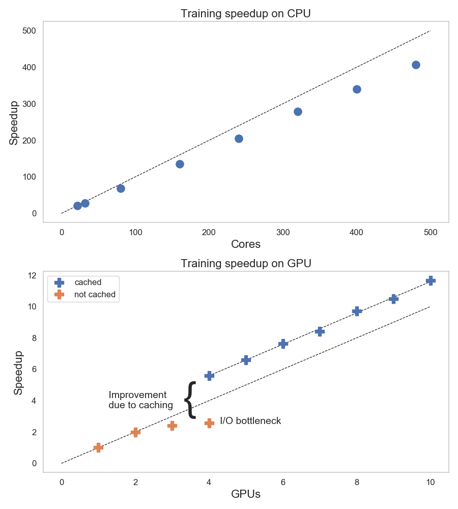
Figure 2: Measured speedup for the distributed training of the Inclusive Classifier model using TensorFlow and tf.distribute with “multi  worker  mirror  strategy”, running on cloud resources with CPU and GPU nodes (Nvidia P100), training for 6 epochs. The speedup values indicate how well the distributed training scales as the number of worker nodes, with CPU and GPU resources, increases.
  

Results and Performance Measurements, CPU and GPU Tests

  
We deployed our tests using Oracle's OCI. Cloud resources were used to build Kubernetes clusters using virtual machines (VMs). We used a set of Terraform script to automate the configuration process. The cluster for CPU tests used VMs of the flavor "VM.Standard2.16'', based on 2.0 GHz Intel Xeon Platinum 8167M, each providing 16 physical cores (Oracle cloud refers to this as OCPUs) and 240 GB of RAM. Tests in our configuration deployed 3 pods for each VM (Kubernetes node), each pod running one TensorFlow worker. Additional OS-based measurements on the VMs confirmed that this was a suitable configuration, as we could measure that the CPU utilization on each VM matched the number of available physical cores (OCPUs), therefore providing good utilization without saturation. The available RAM in the worker nodes was used to cache the training dataset using the tf.data API (data populates the cache during the first epoch).
Figure 2 shows the results of the Inclusive Classifier model training speedup for a variable number of nodes and CPU cores. Tests have been run using TF-Spawner. Measurements show that the training time decreases as the number of allocated cores increases. The speedup grows close to linearly in the range tested: from 32 cores to 480 cores. The largest distributed training test that we ran using CPU, used 480 physical cores (OCPU), distributed over 30 VM, each running 3 workers each (each worker running in a separate container in a pod), for a total of 90 workers.

Similarly, we have performed tests using GPU resources on OCI and running the workload with TF-Spawner. For the GPU tests we have used the VM flavor "GPU 2.1'' which comes equipped with one Nvidia P100 GPU, 12 physical cores (OCPU) and 72 GB of RAM. We have tested with distributed training up to 10 GPUs, and found that scalability was close to linear in the tested range. One important lesson learned when using GPUs is, that the slow performance of reading data from OCI storage makes the first training epoch much slower than the rest of the epochs (up to 3-4 times slower). It was therefore very important to use TensorFlow's caching for the training dataset for our tests with GPUs. However, we could only cache the training dataset for tests using 4 nodes or more, given the limited amount of memory in the VM flavor used (72 GB of RAM per node) compared to the size of the training set (200 GB).
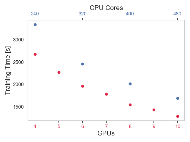
Distributed training tests with CPUs and GPUs were performed using the same infrastructure, namely a Kubernetes cluster built on cloud resources and cloud storage allocated on OCI. Moreover, we used the same script for CPU and GPU training and used the same APIs, tf.distribute and tf.keras, and the same TensorFlow version. The TensorFlow runtime used was different for the two cases, as training on GPU resources took advantage of TensorFlow's optimizations for CUDA and Nvidia GPUs. Figure 3 shows the distributed training time measured for some selected cluster configurations. We can use these results to compare the performance we found when training on GPU and on CPU. For example, we find in Figure 3 that the training time of the Inclusive Classifier for 6 epochs using 400 CPU cores (distributed over 25 VMs equipped with 16 physical cores each) is about 2000 seconds, which is similar to the training time we measured when distributing the training over 6 nodes equipped with GPUs.
When training using GPU resources (Nvidia P100), we measured that each batch is processed in about 59 ms (except for epoch 1 which is I/O bound and is about 3x slower). Each batch contains 128 records, and has a size of about 7.4 MB. This corresponds to a measured throughput of training data flowing through the GPU of about 125 MB/sec per node (i.e. 1.2 GB/sec when training using 10 GPUs). When training on CPU, the measured processing time per batch is about 930 ms, which corresponds to 8 MB/sec per node, and amounts to 716 MB/sec for the training test with 90 workers and 480 CPU cores.
We do not believe these results can be easily generalized to other environments and models, however, they are reported here as they can be useful as an example and for future reference.

Figure 3: Selected measurements of the distributed training time for the Inclusive Classifier model using TensorFlow and tf.distribute with “multi worker mirror strategy”, training for 6 epochs, running on cloud resources, using CPU (2.0 GHz Intel Xeon Platinum 8167M) and GPU (Nvidia P100) nodes, on Oracle's OCI.

TF-Spawner

  
TF-Spawner is an experimental tool for running TensorFlow distributed training on Kubernetes clusters.
TF-Spawner takes as input the user's Python code for TensorFlow training, which is expected to use tf.distribute strategy for multi worker training, and runs it on a Kubernetes cluster. TF-Spawner takes care of requesting the desired number of workers, each running in a container image inside a dedicated pod (unit of execution) on a Kubernetes cluster. We used the official TensorFlow images from Docker Hub for this work. Moreover, TF-Spawner handles the distribution of the necessary credentials for authenticating with cloud storage and manages the TF_CONFIG environment variable needed by tf.distribute.

Examples:


TensorBoard  metrics visualization:

TensorBoard provides monitoring and instrumentation for TensorFlow operations. To use TensorBoard with TF-Spawner you can follow a few additional steps detailed in the documentation.

Figure 4: TensorBoard visualization of the distributed training metrics for the Inclusive Classifier, trained on 10 GPUs nodes on a Kubernetes cluster using TF-Spawner. Measurements show that training convergences smoothly. Note: the reason why we see lower accuracy and greater loss for the training dataset compared to the validation dataset is due to the use of dropout in the model.

Limitations: We found TF-Spawner powerful and easy to use for the scope of this work. However, it is an experimental tool. Notably, there is no validation of the user-provided training script, it is simply passed to Python for execution. Users need to make sure that all the requested pods are effectively running, and have to manually take care of possible failures. At the end of the training, the pods will be found in "Completed" state, users can then manually get the information they need, such as the training time from the pods' log files. Similarly, other common operations, such as fetching the saved trained model, or monitoring training with TensorBoard, will need to be performed manually. These are all relatively easy tasks, but require additional effort and some familiarity with the Kubernetes environment.
Another limitation to the proposed approach is that the use of TF-Spawner does not naturally fit with the use of Jupyter Notebooks, which are often the preferred environment for ML development. Ideas for future work in this direction and other tools that can be helpful in this area are listed in the conclusions.
If you try and find TF-Spawner useful for your work, we welcome feedback.

Conclusions and Acknowledgements

  
This work shows an example of how we implemented distributed deep learning for a High Energy Physics use case, using commonly used tools and platforms from industry and open source, namely TensorFlow and Kubernetes. A key point of this work is demonstrating the use of cloud resources to scale out distributed training.
Machine learning and deep learning on large amounts of data are standard tools for particle physics, and their use is expected to increase in the HEP community in the coming year, both for data acquisition and for data analysis workflows, notably in the context of the challenges of the High Luminosity LHC project. Improvements in productivity and cost reduction for development, deployment, and maintenance of machine learning pipelines on HEP data are of high interest.
We have developed and used a simple tool for running TensorFlow distributed training on Kubernetes clusters, TF-Spawner. Previously reported work has addressed the implementation of the pipeline and distributed training using Apache Spark. Future work may address the use of other solutions for distributed training, using cloud resources and open source tools, such as Horovod on Spark and KubeFlow. In particular, we are interested in further exploring the integration of distributed training with the analytics platforms based on Jupyter Notebooks.

This work has been developed in the context of the Data Analytics services at CERN and of the CERN openlab project on machine learning in the cloud in collaboration with Oracle. Additional information on the work described here can be found in the article Machine Learning Pipelines with Modern Big DataTools for High Energy Physics. The authors would like to thank Matteo Migliorini and Marco Zanetti of the University of Padova for their collaboration and joint work, Thong Nguyen and Maurizio Pierini for their  help, suggestions, and for providing the dataset and models for this work. Many thanks also to CERN openlab, to our Oracle contacts for this project, and to our colleagues at the Spark and Hadoop Service at CERN.