Showing posts with label tools. Show all posts

Monday, September 8, 2025

Troubleshoot I/O & Wait Latency with OraLatencyMap and PyLatencyMap

I recently chased an Oracle performance issue where most reads were sub-millisecond (cache), but a thin band around ~10 ms (spindles) dominated total wait time. Classic bimodal latency: the fast band looked fine in averages, yet the rare slow band owned the delay.

To investigate, and prove it, I refreshed two of my old tools:

  • OraLatencyMap (SQL*Plus script): samples Oracle’s microsecond wait-event histograms and renders two terminal heat maps with wait event latency details over time

  • PyLatencyMap (Python): a general latency heat-map visualizer that reads record-oriented histogram streams from Oracle scripts, BPF/bcc, SystemTap, DTrace, trace files, etc.

Both now have fresh releases with minor refactors and dependency checks.

Friday, April 26, 2024

Building an Apache Spark Performance Lab: Tools and Techniques for Spark Optimization

Apache Spark is renowned for its speed and efficiency in handling large-scale data processing. However, optimizing Spark to achieve maximum performance requires a precise understanding of its inner workings. This blog post will guide you through establishing a Spark Performance Lab with essential tools and techniques aimed at enhancing Spark performance through detailed metrics analysis.

Why a Spark Performance Lab

The purpose of a Spark Performance Lab isn't just to measure the elapsed time of your Spark jobs but to understand the underlying performance metrics deeply. By using these metrics, you can create models that explain what's happening within Spark's execution and identify areas for improvement. Here are some key reasons to set up a Spark Performance Lab:

  • Hands-on learning and testing: A controlled lab setting allows for safer experimentation with Spark configurations and tuning and also experimenting and understanding the monitoring tools and Spark-generated metrics.
  • Load and scale: Our lab uses a workload generator, running TPCDS queries. This is a well-known set of complex queries that is representative of OLAP workloads, and that can easily be scaled up for testing from GBs to 100s of TBs.
  • Improving your toolkit: Having a toolbox is invaluable, however you need to practice and understand their output in a sandbox environment before moving to production.
  • Get value from the Spark metric system: Instead of focusing solely on how long a job takes, use detailed metrics to understand the performance and spot inefficiencies.

Tools and Components

In our Spark Performance Lab, several key tools and components form the backbone of our testing and monitoring environment:

  • Workload generator: 
    • We use a custom tool, TPCDS-PySpark, to generate a consistent set of queries (TPCDS benchmark), creating a reliable testing framework.
  • Spark instrumentation: 
    • Spark’s built-in Web UI for initial metrics and job visualization.
  • Custom tools:
    • SparkMeasure: Use this for detailed performance metrics collection.
    • Spark-Dashboard: Use this to monitor Spark jobs and visualize key performance metrics.

Additional tools for Performance Measurement include:

Demos

These quick demos and tutorials will show you how to use the tools in this Spark Performance Lab. You can follow along and get the same results on your own, which will help you start learning and exploring.


Figure 1: The graph illustrates the dynamic task allocation in a Spark application during a TPCDS 10TB benchmark on a YARN cluster with 256 cores. It showcases the variability in the number of active tasks over time, highlighting instances of execution "long tails" and straggler tasks, as seen in the periodic spikes and troughs.

How to Make the Best of Spark Metrics System

Understanding and utilizing Spark's metrics system is crucial for optimization:
  • Importance of Metrics: Metrics provide insights beyond simple timing, revealing details about task execution, resource utilization, and bottlenecks.

  • Execution Time is Not Enough: Measuring the execution time of a job (how long it took to run it), is useful, but it doesn’t show the whole picture. Say the job ran in 10 seconds. It's crucial to understand why it took 10 seconds instead of 100 seconds or just 1 second. What was slowing things down? Was it the CPU, data input/output, or something else, like data shuffling? This helps us identify the root causes of performance issues.

  • Key Metrics to Collect:
    • Executor Run Time: Total time executors spend processing tasks.
    • Executor CPU Time: Direct CPU time consumed by tasks.
    • JVM GC Time: Time spent in garbage collection, affecting performance.
    • Shuffle and I/O Metrics: Critical for understanding data movement and disk interactions.
    • Memory Metrics: Key for performance and troubleshooting Out Of Memory errors.

  • Metrics Analysis, what to look for:
    • Look for bottlenecks: are there resources that are the bottleneck? Are the jobs running mostly on CPU or waiting for I/O or spending a lot of time on Garbage Collection?
    • USE method: Utilization Saturation and Errors (USE) Method is a methodology for analyzing the performance of any system. 
      • The tools described here can help you to measure and understand Utilization and Saturation.
    • Can your job use a significant fraction of the available CPU cores? 
      • Examine the measurement of  the actual number of active tasks vs. time.
      • Figure 1 shows the number of active tasks measured while running TPCDS 10TB on a YARN cluster, with 256 cores allocated. The graph shows spikes and troughs.
      • Understand the root causes of the troughs using metrics and monitoring data. The reasons can be many: resource allocation, partition skew, straggler tasks, stage boundaries, etc.
    • Which tool should I use?
      • Start with using the Spark Web UI
      • Instrument your jobs with sparkMesure. This is recommended early in the application development, testing, and for Continuous Integration (CI) pipelines.
      • Observe your Spark application execution profile with Spark-Dashboard.
      • Use available tools with OS metrics too. See also Spark-Dashboard extended instrumentation: it collects and visualizes OS metrics (from cgroup statistics) like network stats, etc
    • Drill down:
Figure 2: This technical drawing outlines the integrated monitoring pipeline for Apache Spark implemented by Spark-Dashboard using open-source components. The flow of the diagram illustrates the Spark metrics source and the components used to store and visualize the metrics.


Lessons Learned and Conclusions

From setting up and running a Spark Performance Lab, here are some key takeaways:

  • Collect, analyze and visualize metrics: Go beyond just measuring jobs' execution times to troubleshoot and fine-tune Spark performance effectively.
  • Use the Right Tools: Familiarize yourself with tools for performance measurement and monitoring.
  • Start Small, Scale Up: Begin with smaller datasets and configurations, then gradually scale to test larger, more complex scenarios.
  • Tuning is an Iterative Process: Experiment with different configurations, parallelism levels, and data partitioning strategies to find the best setup for your workload.

Establishing a Spark Performance Lab is a fundamental step for any data engineer aiming to master Spark's performance aspects. By integrating tools like Web UI, TPCDS_PySpark, sparkMeasure, and Spark-Dashboard, developers and data engineers can gain unprecedented insights into Spark operations and optimizations. 

Explore this lab setup to turn theory into expertise in managing and optimizing Apache Spark. Learn by doing and experimentation!

Acknowledgements: A special acknowledgment goes out to the teams behind the CERN data analytics, monitoring, and web notebook services, as well as the dedicated members of the ATLAS database group.


Friday, August 28, 2020

Apache Spark 3.0 Memory Monitoring Improvements

TLDR; Apache Spark 3.0 comes with many improvements, including new features for memory monitoring. This can help you troubleshooting memory usage and optimizing the memory configuration of your Spark jobs for better performance and stability, see SPARK-23429 and SPARK-27189.

The problem with memory
Memory is key for the performance and stability of Spark jobs. If you don't allocate enough memory for your Spark executors you are more likely to run into the much dreaded Java OOM (out of memory) errors or substantially degrade your jobs' performance. Memory is needed by Spark to execute efficiently Dataframe/RDD operations, and for improving the performance of algorithms that would otherwise have to swap to disk in their processing (e.g. shuffle operations), moreover, it can be used for caching data, reducing I/O. This is all good in theory, but in practice how do you know how much memory you need?

A basic solution
One first basic approach to memory sizing for Spark jobs, is to start by giving the executors ample amounts of memory, provided your systems has enough resources. For example, by setting the spark.executor.memory configuration parameter to several GBs. Note, in local mode you would set sprk.driver.memory instead. You can further tune the configuration by trial-and-error, by reducing and increasing memory with each test and observe the results. This approach may give good results quickly, but it is not a very solid approach to the problem.

A more structured approach to memory usage troubleshooting and to sizing memory for Spark jobs is to use monitoring data to understand how much memory is used by the Spark application, which jobs request more memory, and which memory areas are used, finally linking this back to the application details and in the context of other resources utilization (for example, CPU usage).
This approach helps with drilling down on issues of OOM, and also to be more precise in allocating memory for Spark applications, aiming at using just enough memory as needed, without wasting memory that can be a scarce shared resource in some systems. It is still an experimental and iterative process, but more informed than the basic trial-and-error solution.

How memory is allocated and used by Spark

Configuration of executor memory

The main configuration parameter used to request the allocation of executor memory is spark.executor.memory.Spark running on YARN, Kubernetes or Mesos, adds to that a memory overhead  to cover for additional memory usage (OS, redundancy, filesystem cache, off-heap allocations, etc), which is calculated as memory_overhead_factor * spark.executor.memory  (with a minimum of 384 MB). The overhead factor is 0.1 (10%), it can be configured when running on Kubernetes (only) using spark.kubernetes.memoryOverheadFactor.
When using PySpark additional memory can be allocated using spark.executor.pyspark.memory
Additional memory for off-heap allocation is configured using spark.memory.offHeap.size=<size> and spark.memory.offHeap.enabled=true. This works on YARN, for K8S, see SPARK-32661.  
Note also parameters for driver memory allocation: spark.driver.memory and spark.driver.memoryOverhead
Note: this covers recent versions of Spark at the time of this writing, notably Spark 3.0 and 2.4. See also Spark documentation.
  
Figure 1: Pictorial representation of the memory areas allocated and used by Spark executors and the main parameters for their configuration. 
  

Spark unified memory pool

Spark tasks allocate memory for execution and storage from the JVM heap of the executors using a unified memory pool managed by the Spark memory management systemUnified memory occupies by default 60% of the JVM heap: 0.6 * (spark.executor.memory - 300 MB). The factor 0.6 (60%) is the default value of the configuration parameter spark.memory.fraction. 300MB is a hard-coded value of "reserved memory". The rest of the memory is used for user data structures, internal metadata in Spark, and safeguarding against OOM errors. 
Spark manages execution and storage memory requests using the unified memory pool. When little execution memory is used, storage can acquire most of the available memory, and vice versa. Additional structure in the working of the storage and execution memory is exposed with the configuration parameter spark.memory.storageFraction (default is 0.5), which guarantees that the stored blocks will not be evicted from the unified memory by execution below the specified threshold.
The unified memory pool can optionally be allocated using off-heap memory, the relevant configuration parameters are: spark.memory.offHeap.size and spark.memory.offHeap.enabled
  

Opportunities for memory configuration settings

The first key configuration to get right is spark.executor.memory. Monitoring data (see the following paragraphs) can help you understand if you need to increase the memory allocated to Spark executors and or if you are already allocating plenty of memory and can consider reducing the memory footprint.
There are other memory-related configuration parameters that may need some adjustments for specific workloads: this can be analyzed and tested using memory monitoring data.
In particular, increasing spark.memory.fraction (default is 0.6) may be useful when deploying large Java heap, as there is a chance that you will not need to set aside 40% of the JVM heap for user memory. With similar reasoning, when using large Java heap allocation, manually setting spark.executor.memoryOverhead to a value lower than the default (0.1 * spark.executor.memory) can be tested.
  

Memory monitoring improvements in Spark 3.0

Two notable improvements in Spark 3.0 for memory monitoring are:
  • SPARK-23429: Add executor memory metrics to heartbeat and expose in executors REST API
    • see also the umbrella ticket SPARK-23206: Additional Memory Tuning Metrics
  • SPARK-27189: Add Executor metrics and memory usage instrumentation to the metrics system
When troubleshooting memory usage it is important to investigate how much memory was used as the workload progresses and measure peak values of memory usage. Peak values are particularly important, as this is where you get possible slow downs or even OOM errors. Spark 3.0 instrumentation adds monitoring data on the amount of memory used, drilling down on unified memory, and memory used by Python (when using PySpark). This is implemented using a new set of metrics called "executor metrics", and can be helpful for memory sizing and troubleshooting performance. 
    

Measuring memory usage and peak values using the REST API

An example of the data you can get from the REST API in Spark 3.0:

WebUI URL + /api/v1/applications/<application_id>/executors

Here below you can find a snippet of the peak executor memory metrics, sampled on a snapshot and limited to one of the executors used for testing:
"peakMemoryMetrics" : {
    "JVMHeapMemory" : 29487812552,
    "JVMOffHeapMemory" : 149957200,
    "OnHeapExecutionMemory" : 12458956272,
    "OffHeapExecutionMemory" : 0,
    "OnHeapStorageMemory" : 83578970,
    "OffHeapStorageMemory" : 0,
    "OnHeapUnifiedMemory" : 12540212490,
    "OffHeapUnifiedMemory" : 0,
    "DirectPoolMemory" : 66809076,
    "MappedPoolMemory" : 0,
    "ProcessTreeJVMVMemory" : 38084534272,
    "ProcessTreeJVMRSSMemory" : 36998328320,
    "ProcessTreePythonVMemory" : 0,
    "ProcessTreePythonRSSMemory" : 0,
    "ProcessTreeOtherVMemory" : 0,
    "ProcessTreeOtherRSSMemory" : 0,
    "MinorGCCount" : 561,
    "MinorGCTime" : 49918,
    "MajorGCCount" : 0,
    "MajorGCTime" : 0
  },

Notes:
  • Procfs metrics (SPARK-24958) provide a view on the process usage from "the OS point of observation".
    • Notably, procfs metrics provide a way to measure memory usage by Python, when using PySpark and in general other processes that may be spawned by Spark tasks.
  • Profs metrics are gathered conditionally:
    • if the /proc filesystem exists
    • if spark.executor.processTreeMetrics.enabled=true
    • The optional configuration spark.executor.metrics.pollingInterval allows to gather executor metrics at high frequency, see doc.
  • Additional improvements of the memory instrumentation via REST API (targeting Spark 3.1) are in "SPARK-23431 Expose the new executor memory metrics at the stage level".
  

Improvements to the Spark metrics system and Spark performance dashboard

The Spark metrics system based on the Dropwizard metrics library provides the data source to build a Spark performance dashboard. A dashboard naturally leads to time series visualization of Spark performance and workload metrics. Spark 3.0 instrumentation (SPARK-27189) hooks to the executor metrics data source and makes available the time series data with the evolution of memory usage. 
Some of the advantages of collecting metrics values and visualizing them with Grafana are:
  • The possibility to see the evolution of the metrics values in real time and to compare them with other key metrics of the workload. 
  • Metrics can be examined as aggregated values or drilled down at the executor level. This allows you to understand if there are outliers or stragglers.
  • It is possible to study the evolution of the metrics values with time and understand which part of the workload has generated certain spikes in a given metric, for example. It is also possible to annotate the dashboard graphs, as explained at this link, with details of query id, job id, and stage id.
Here are a few examples of dashboard graphs related to memory usage:


Figure 2: Graphs of memory-related  metrics collected and visualized using a Spark performance dashboard. Metrics reported in the figure are: Java heap memory, RSS memory, Execution memory, and Storage memory. The Grafana dashboard allows us to drill down on the metrics values per executor. These types of plots can be used to study the time evolution of key metrics.
  

What if you are using Spark 2.x?

Some monitoring features related to memory usage are already available in Spark 2.x and still useful in Spark 3.0:
  • Task metrics are available in the REST API and in the dropwizard-based metrics and provide information:
    • Garbage Collection time: when garbage collection takes a significant amount of time typically you want to investigate for the need for allocating more memory (or reducing memory usage).
    • Shuffle-related metrics: memory can prevent some shuffle operations with I/O to storage and be beneficial for performance.
    • Task peak execution memory metric.
  • The WebUI reports storage memory usage per executor.
  • Spark dropwizard-based metrics system provides a JVM source with memory-related utilization metrics.


Lab configuration:

When experimenting and trying to get a grasp for the many parameters related to memory and monitoring, I found it useful to set up a small test workload. Some notes on the setup I used:


bin/spark-shell --master yarn --num-executors 16 --executor-cores 8 \
--driver-memory 4g --executor-memory 32g \
--jars /home/luca/spark-sql-perf/target/scala-2.12/spark-sql-perf_2.12-0.5.1-SNAPSHOT.jar \
--conf spark.eventLog.enabled=false \
--conf spark.sql.shuffle.partitions=512 \
--conf spark.sql.autoBroadcastJoinThreshold=100000000 \
--conf spark.executor.processTreeMetrics.enabled=true
  
  
import com.databricks.spark.sql.perf.tpcds.TPCDSTables
val tables = new TPCDSTables(spark.sqlContext, "/home/luca/tpcds-kit/tools","1500")
tables.createTemporaryTables("/project/spark/TPCDS/tpcds_1500_parquet_1.10.1", "parquet")
val tpcds = new com.databricks.spark.sql.perf.tpcds.TPCDS(spark.sqlContext)
val experiment = tpcds.runExperiment(tpcds.tpcds2_4Queries)


Limitations and caveats

  • Spark metrics and instrumentation are still an area in active development. There is room for improvement both in their implementation and documentation. I found that some of the metrics may be difficult to understand or may present what looks like strange behaviors in some circumstances. In general, more testing and sharing experience between Spark users may be highly beneficial for further improving Spark instrumentation.
  • The tools and methods discussed here are based on metrics, they are reactive by nature, and suitable for troubleshooting and iterative experimentation.
  • This post is centered on  describing Spark 3.0 new features for memory monitoring and how you can experiment with them. A key piece left for future work is to show some real-world examples of troubleshooting using memory metrics and instrumentation.
  • For the scope of this post, we assume that the workload to troubleshoot is a black box and that we just want to try to optimize the memory allocation  and use. This post does not cover techniques to improve the memory footprint of Spark jobs, however, they are very important for correctly using Spark. Examples of techniques that are useful in this area are: implementing the correct partitioning scheme for the data and operations, reducing partition skew, using the appropriate join mechanisms, streamlining caching, and many others, covered elsewhere. 
  

References

Talks:
Spark documentation and blogs:

JIRAs:  SPARK-23206SPARK-23429 and SPARK-27189 contain most of the details of the improvements in Apache Spark discussed here.


Conclusions and acknowledgments

It is important to correctly size memory configurations for Spark applications. This improves performance, stability, and resource utilization in multi-tenant environments. Spark 3.0 has important improvements to memory monitoring instrumentation. The analysis of peak memory usage, and of memory use broken down by area and plotted as a function of time, provide important insights for troubleshooting OOM errors and for Spark job memory sizing.   
Many thanks to the Apache Spark community, and in particular the committers and reviewers who have helped with the improvements in SPARK-27189.
This work has been developed in the context of the data analytics services at CERN, many thanks to my colleagues for help and suggestions.  
  

Thursday, March 26, 2020

Distributed Deep Learning for Physics with TensorFlow and Kubernetes

Summary: This post details a solution for distributed deep learning training for a High Energy Physics use case, deployed using cloud resources and Kubernetes. You will find the results for training using CPU and GPU nodes. This post also describes an experimental tool that we developed, TF-Spawner, and how we used it to run distributed TensorFlow on a Kubernetes cluster.

Authors: Riccardo.Castellotti@cern.ch and Luca.Canali@cern.ch

A Particle Classifier

  
This work was developed as part of the pipeline described in Machine Learning Pipelines with Modern Big DataTools for High Energy Physics. The main goal is to build a particle classifier to improve the quality of data filtering for online systems at the LHC experiments. The classifier is implemented using a neural network model described in this research article.
The datasets used for test and training are stored in TFRecord format, with a cumulative size of about 250 GB, with 34 million events in the training dataset. A key part of the neural network (see Figure 1) is a GRU layer that is trained using lists of 801 particles with 19 low-level features each, which account for most of the training dataset. The datasets used for this work have been produced using Apache Spark, see details and code. The original pipeline produces files in Apache Parquet format; we have used Spark and the spark-tensorflow-connector to convert the datasets into TFRecord format, see also the code.

Data: download the datasets used for this work at this link
Code: see the code used for the tests reported in this post at this link


Figure 1: (left) Diagram of the neural network for the Inclusive Classifier model, from T. Nguyen et. al. (right) TF.Keras implementation used in this work.

Distributed Training on Cloud Resources

  
Cloud resources provide a suitable environment for scaling distributed training of neural networks. One of the key advantages of using cloud resources is the elasticity of the platform that allows allocating resources when needed. Moreover, container orchestration systems, in particular Kubernetes, provide a powerful and flexible API for deploying many types of workloads on cloud resources, including machine learning and data processing pipelines. CERN physicists, and data scientists in general, can access cloud resources and Kubernetes clusters via the CERN OpenStack private cloud. The use of public clouds is also being actively tested for High Energy Physics (HEP) workloads. The tests reported here have been run using resources from Oracle's OCI.
For this work, we have developed a custom launcher script, TF-Spawner (see also the paragraph on TF-Spawner for more details) for running distributed TensorFlow training code on Kubernetes clusters.
Training and test datasets have been copied to the cloud object storage prior to running the tests, OCI object storage in this case, while for tests run at CERN we used an S3 installation based on Ceph. Our model training job with TensorFlow used training and test data in TFRecord format, produced at the end of the data preparation part of the pipeline, as discussed in the previous paragraph. TensorFlow reads natively TFRecord format and has tunable parameters and optimizations when ingesting this type of data using the modules tf.data and tf.io. We found that reading from OCI object storage can become a bottleneck for distributed training, as it requires reading data over the network which can suffer from bandwidth saturation, latency spikes and/or multi-tenancy noise. We followed TensorFlow's documentation recommendations for improving the data pipeline performance, by using prefetching, parallel data extraction, sequential interleaving, caching, and by using a large read buffer. Notably, caching has proven to be very useful for distributed training with GPUs and for some of the largest tests on CPU, where we observed that the first training epoch, which has to read the data into the cache, was much slower than subsequent epoch which would find data already cached.
Tests were run using TensorFlow version 2.0.1, using tf.distribute strategy "multi worker mirror strategy''. Additional care was taken to make sure that the different tests would also yield the same good results in terms of accuracy on the test dataset as what was found with training methods tested in previous work. To achieve this we have found that additional tuning was needed on the settings of the learning rate for the optimizer (we use the Adam optimizer for all the tests discussed in this article). We scaled the learning rate with the number of workers, to match the increase in effective batch size (we used 128 for each worker). In addition, we found that slowly reducing the learning rate as the number of epochs progressed, was beneficial to the convergence of the network. This additional step is an ad hoc tuning that we developed by trial and error and that we validated by monitoring the accuracy and loss on the test dataset at the end of each training.
To gather performance data, we ran the training for 6 epochs, which provided accuracy and loss very close to the best results that we would obtain by training the network up to 12 epochs. We have also tested adding shuffling between each epoch, using the shuffle method of the tf.data API, however it has not shown measurable improvements so this technique has not been further used in the tests reported here.

Figure 2: Measured speedup for the distributed training of the Inclusive Classifier model using TensorFlow and tf.distribute with “multi  worker  mirror  strategy”, running on cloud resources with CPU and GPU nodes (Nvidia P100), training for 6 epochs. The speedup values indicate how well the distributed training scales as the number of worker nodes, with CPU and GPU resources, increases.
  

Results and Performance Measurements, CPU and GPU Tests

  
We deployed our tests using Oracle's OCI. Cloud resources were used to build Kubernetes clusters using virtual machines (VMs). We used a set of Terraform script to automate the configuration process. The cluster for CPU tests used VMs of the flavor "VM.Standard2.16'', based on 2.0 GHz Intel Xeon Platinum 8167M, each providing 16 physical cores (Oracle cloud refers to this as OCPUs) and 240 GB of RAM. Tests in our configuration deployed 3 pods for each VM (Kubernetes node), each pod running one TensorFlow worker. Additional OS-based measurements on the VMs confirmed that this was a suitable configuration, as we could measure that the CPU utilization on each VM matched the number of available physical cores (OCPUs), therefore providing good utilization without saturation. The available RAM in the worker nodes was used to cache the training dataset using the tf.data API (data populates the cache during the first epoch).
Figure 2 shows the results of the Inclusive Classifier model training speedup for a variable number of nodes and CPU cores. Tests have been run using TF-Spawner. Measurements show that the training time decreases as the number of allocated cores increases. The speedup grows close to linearly in the range tested: from 32 cores to 480 cores. The largest distributed training test that we ran using CPU, used 480 physical cores (OCPU), distributed over 30 VM, each running 3 workers each (each worker running in a separate container in a pod), for a total of 90 workers.

Similarly, we have performed tests using GPU resources on OCI and running the workload with TF-Spawner. For the GPU tests we have used the VM flavor "GPU 2.1'' which comes equipped with one Nvidia P100 GPU, 12 physical cores (OCPU) and 72 GB of RAM. We have tested with distributed training up to 10 GPUs, and found that scalability was close to linear in the tested range. One important lesson learned when using GPUs is, that the slow performance of reading data from OCI storage makes the first training epoch much slower than the rest of the epochs (up to 3-4 times slower). It was therefore very important to use TensorFlow's caching for the training dataset for our tests with GPUs. However, we could only cache the training dataset for tests using 4 nodes or more, given the limited amount of memory in the VM flavor used (72 GB of RAM per node) compared to the size of the training set (200 GB).
Distributed training tests with CPUs and GPUs were performed using the same infrastructure, namely a Kubernetes cluster built on cloud resources and cloud storage allocated on OCI. Moreover, we used the same script for CPU and GPU training and used the same APIs, tf.distribute and tf.keras, and the same TensorFlow version. The TensorFlow runtime used was different for the two cases, as training on GPU resources took advantage of TensorFlow's optimizations for CUDA and Nvidia GPUs. Figure 3 shows the distributed training time measured for some selected cluster configurations. We can use these results to compare the performance we found when training on GPU and on CPU. For example, we find in Figure 3 that the training time of the Inclusive Classifier for 6 epochs using 400 CPU cores (distributed over 25 VMs equipped with 16 physical cores each) is about 2000 seconds, which is similar to the training time we measured when distributing the training over 6 nodes equipped with GPUs.
When training using GPU resources (Nvidia P100), we measured that each batch is processed in about 59 ms (except for epoch 1 which is I/O bound and is about 3x slower). Each batch contains 128 records, and has a size of about 7.4 MB. This corresponds to a measured throughput of training data flowing through the GPU of about 125 MB/sec per node (i.e. 1.2 GB/sec when training using 10 GPUs). When training on CPU, the measured processing time per batch is about 930 ms, which corresponds to 8 MB/sec per node, and amounts to 716 MB/sec for the training test with 90 workers and 480 CPU cores.
We do not believe these results can be easily generalized to other environments and models, however, they are reported here as they can be useful as an example and for future reference.

Figure 3: Selected measurements of the distributed training time for the Inclusive Classifier model using TensorFlow and tf.distribute with “multi worker mirror strategy”, training for 6 epochs, running on cloud resources, using CPU (2.0 GHz Intel Xeon Platinum 8167M) and GPU (Nvidia P100) nodes, on Oracle's OCI.

TF-Spawner

  
TF-Spawner is an experimental tool for running TensorFlow distributed training on Kubernetes clusters.
TF-Spawner takes as input the user's Python code for TensorFlow training, which is expected to use tf.distribute strategy for multi worker training, and runs it on a Kubernetes cluster. TF-Spawner takes care of requesting the desired number of workers, each running in a container image inside a dedicated pod (unit of execution) on a Kubernetes cluster. We used the official TensorFlow images from Docker Hub for this work. Moreover, TF-Spawner handles the distribution of the necessary credentials for authenticating with cloud storage and manages the TF_CONFIG environment variable needed by tf.distribute.

Examples:


TensorBoard  metrics visualization:

TensorBoard provides monitoring and instrumentation for TensorFlow operations. To use TensorBoard with TF-Spawner you can follow a few additional steps detailed in the documentation.

Figure 4: TensorBoard visualization of the distributed training metrics for the Inclusive Classifier, trained on 10 GPUs nodes on a Kubernetes cluster using TF-Spawner. Measurements show that training convergences smoothly. Note: the reason why we see lower accuracy and greater loss for the training dataset compared to the validation dataset is due to the use of dropout in the model.

Limitations: We found TF-Spawner powerful and easy to use for the scope of this work. However, it is an experimental tool. Notably, there is no validation of the user-provided training script, it is simply passed to Python for execution. Users need to make sure that all the requested pods are effectively running, and have to manually take care of possible failures. At the end of the training, the pods will be found in "Completed" state, users can then manually get the information they need, such as the training time from the pods' log files. Similarly, other common operations, such as fetching the saved trained model, or monitoring training with TensorBoard, will need to be performed manually. These are all relatively easy tasks, but require additional effort and some familiarity with the Kubernetes environment.
Another limitation to the proposed approach is that the use of TF-Spawner does not naturally fit with the use of Jupyter Notebooks, which are often the preferred environment for ML development. Ideas for future work in this direction and other tools that can be helpful in this area are listed in the conclusions.
If you try and find TF-Spawner useful for your work, we welcome feedback.

Conclusions and Acknowledgements

  
This work shows an example of how we implemented distributed deep learning for a High Energy Physics use case, using commonly used tools and platforms from industry and open source, namely TensorFlow and Kubernetes. A key point of this work is demonstrating the use of cloud resources to scale out distributed training.
Machine learning and deep learning on large amounts of data are standard tools for particle physics, and their use is expected to increase in the HEP community in the coming year, both for data acquisition and for data analysis workflows, notably in the context of the challenges of the High Luminosity LHC project. Improvements in productivity and cost reduction for development, deployment, and maintenance of machine learning pipelines on HEP data are of high interest.
We have developed and used a simple tool for running TensorFlow distributed training on Kubernetes clusters, TF-Spawner. Previously reported work has addressed the implementation of the pipeline and distributed training using Apache Spark. Future work may address the use of other solutions for distributed training, using cloud resources and open source tools, such as Horovod on Spark and KubeFlow. In particular, we are interested in further exploring the integration of distributed training with the analytics platforms based on Jupyter Notebooks.

This work has been developed in the context of the Data Analytics services at CERN and of the CERN openlab project on machine learning in the cloud in collaboration with Oracle. Additional information on the work described here can be found in the article Machine Learning Pipelines with Modern Big DataTools for High Energy Physics. The authors would like to thank Matteo Migliorini and Marco Zanetti of the University of Padova for their collaboration and joint work, Thong Nguyen and Maurizio Pierini for their  help, suggestions, and for providing the dataset and models for this work. Many thanks also to CERN openlab, to our Oracle contacts for this project, and to our colleagues at the Spark and Hadoop Service at CERN.


Friday, August 24, 2018

SparkMeasure, a tool for performance troubleshooting of Apache Spark workloads

SparkMeasure 

  SparkMeasure simplifies the collection and analysis of Spark task metrics data. It is also intended as a working example of how to use Spark listeners for collecting and processing Spark performance metrics.
The work on sparkMeasure has been previously presented in this blog with examples. Recently, an updated version of sparkMeasure (version 0.13) introduces additional integration for the PySpark and Jupyter environments, improved documentation and additional features provided by the community via PRs (many thanks to the contributors).
At CERN Spark and Hadoop service we have been using sparkMeasure in a few occasions and found it useful for understanding the performance characteristics of Spark workloads and for performance troubleshooting.
 

Download and deploy with examples

You can find sparkMeasure, its documentation with examples in the sparkMeasure development repository on GitHub and/or in its mirror cerndb repo.
You can deploy sparkMeasure from Maven Central or build with "sbt package". PySpark users can find the Python wrapper API on PyPI: "pip install sparkmeasure".

Use sparkMeasure for measuring interactive and batch workloads

  • Interactive: measure and analyze performance from shell or notebooks: using spark-shell (Scala), PySpark (Python) or Jupyter notebooks.
  • Code instrumentation: add calls in your code to deploy sparkMeasure custom Spark listeners and/or use the classes StageMetrics/TaskMetrics and related APIs for collecting, analyzing and saving metrics data.
  • "Flight Recorder" mode: this records all performance metrics automatically and saves data for later processing.

Documentation and examples


Architecture diagram

sparkMeasure architecture diagram
 

 Main concepts underlying sparkMeasure

  • The tool is based on the Spark Listener interface. Listeners transport Spark executor Task Metrics data from the executor to the driver. They are a standard part of Spark instrumentation, used by the Spark Web UI and History Server for example.
  • Metrics can be collected using sparkMeasure at the granularity of stage completion and/or task completion (configurable)
  • Metrics are flattened and collected into local memory structures in the driver (ListBuffer of a custom case class).
  • Spark DataFrame and SQL are used to further process metrics data for example to generate reports.
  • Metrics data and reports can be saved for offline analysis.
 

Getting started examples of sparkMeasure usage

  1. Link to an example Python_Jupyter Notebook
  2. Example notebooks on the Databricks platform (community edition): example Scala notebook on Databricks, example Python notebook on Databricks
  3. An example using Scala REPL/spark-shell:
bin/spark-shell --packages ch.cern.sparkmeasure:spark-measure_2.11:0.13

val stageMetrics = ch.cern.sparkmeasure.StageMetrics(spark) 
stageMetrics.runAndMeasure(spark.sql("select count(*) from range(1000) cross join range(1000) cross join range(1000)").show())
The output should look like this:
Scheduling mode = FIFO
Spark Context default degree of parallelism = 8
Aggregated Spark stage metrics:
numStages => 3
sum(numTasks) => 17
elapsedTime => 9103 (9 s)
sum(stageDuration) => 9027 (9 s)
sum(executorRunTime) => 69238 (1.2 min)
sum(executorCpuTime) => 68004 (1.1 min)
sum(executorDeserializeTime) => 1031 (1 s)
sum(executorDeserializeCpuTime) => 151 (0.2 s)
sum(resultSerializationTime) => 5 (5 ms)
sum(jvmGCTime) => 64 (64 ms)
sum(shuffleFetchWaitTime) => 0 (0 ms)
sum(shuffleWriteTime) => 26 (26 ms)
max(resultSize) => 17934 (17.0 KB)
sum(numUpdatedBlockStatuses) => 0
sum(diskBytesSpilled) => 0 (0 Bytes)
sum(memoryBytesSpilled) => 0 (0 Bytes)
max(peakExecutionMemory) => 0
sum(recordsRead) => 2000
sum(bytesRead) => 0 (0 Bytes)
sum(recordsWritten) => 0
sum(bytesWritten) => 0 (0 Bytes)
sum(shuffleTotalBytesRead) => 472 (472 Bytes)
sum(shuffleTotalBlocksFetched) => 8
sum(shuffleLocalBlocksFetched) => 8
sum(shuffleRemoteBlocksFetched) => 0
sum(shuffleBytesWritten) => 472 (472 Bytes)
sum(shuffleRecordsWritten) => 8
  

FAQ

  • Why measuring performance with workload metrics instrumentation rather than just using time?
    • Measuring elapsed time, treats your workload as "a black box" and most often does not allow you to understand the root cause of the performance. With workload metrics you can (attempt to) go further in understanding and root cause analysis, bottleneck identification, resource usage measurement.
  • What are Apache Spark tasks metrics and what can I use them for?
    • Apache Spark measures several details of each task execution, including run time, CPU time, information on garbage collection time, shuffle metrics and on task I/O. See also this short description of the Spark Task Metrics
  • How is sparkMeasure different from Web UI/Spark History Server and EventLog?
    • sparkMeasure uses the same ListenerBus infrastructure used to collect data for the Web UI and Spark EventLog.
      • Spark collects metrics and other execution details and exposes them via the Web UI.
      • Notably Task execution metrics are also available through the REST API
      • In addition Spark writes all details of the task execution in the EventLog file (see config of spark.eventlog.enabled and spark.eventLog.dir)
      • The EventLog is used by the Spark History server + other tools and programs can read and parse the EventLog file(s) for workload analysis and performance troubleshooting, see a proof-of-concept example of reading the EventLog with Spark SQL
    • There are key differences that motivate this development:
      • sparkmeasure can collect data at the stage completion-level, which is more lightweight than measuring all the tasks, in case you only need to compute aggregated performance metrics. When needed, sparkMeasure can also collect data at the task granularity level.
      • sparkmeasure has an API that makes it simple to add instrumention/performance measurements in notebooks and application code.
      • sparkmeasure collects data in a flat structure, which makes it natural to use Spark SQL for workload data processing, which provides a simple and powerful interface
      • limitations: sparkMeasure does not collect all the data available in the EventLog, sparkMeasure buffers data in the driver memory, see also the TODO and issues doc
  • What are known limitations and gotchas?
    • The currently available Spark task metrics can give you precious quantitative information on resources used by the executors, however there do not allow to fully perform time-based analysis of the workload performance, notably they do not expose the time spent doing I/O or network traffic.
    • Metrics are collected on the driver, which can be quickly become a bottleneck. This is true in general for ListenerBus instrumentation, in addition sparkMeasure in the current version buffers all data in the driver memory.
    • Task metrics values collected by sparkMeasure are only for successfully executed tasks. Note that resources used by failed tasks are not collected in the current version.
    • Task metrics are collected by Spark executors running on the JVM, resources utilized outside the JVM are currently not directly accounted for (notably the resources used when running Python code inside the python.daemon in the case of PySpark).
  • When should I use stage metrics and when should I use task metrics?
    • Use stage metrics whenever possible as they are much more lightweight. Collect metrics at the task granularity if you need the extra information, for example if you want to study effects of skew, long tails and task stragglers.
  • What are accumulables?
    • Metrics are first collected into accumulators that are sent from the executors to the driver. Many metrics of interest are exposed via [[TaskMetrics]] others are only available in StageInfo/TaskInfo accumulables (notably SQL Metrics, such as "scan time")
  • How can I save/sink the collected metrics?
    • You can print metrics data and reports to standard output or save them to files (local or on HDFS). Additionally you can sink metrics to external systems (such as Prometheus, other sinks like InfluxDB or Kafka may be implemented in future versions).
  • How can I process metrics data?
    • You can use Spark to read the saved metrics data and perform further post-processing and analysis. See the also Notes on metrics analysis.
  • How can I contribute to sparkMeasure?
    • SparkMeasure has already profited from PR contributions. Additional contributions are welcome. See the TODO_and_issues list for a list of known issues and ideas on what you can contribute.
 

Acknowledgements and additional links

This work has been developed in the context of the CERN Hadoop, Spark and Streaming services and of the CERN openlab project on data analytics. Credits go to my colleagues for collaboration. Many thanks also to the Apache Spark community, in particular to the contributors of PRs and reporters of issues. Additional links on this topic are: 

Friday, September 29, 2017

Performance Analysis of a CPU-Intensive Workload in Apache Spark

Topic: This post is about techniques and tools for measuring and understanding CPU-bound and memory-bound workloads in Apache Spark. You will find examples applied to studying a simple workload consisting of reading Apache Parquet files into a Spark DataFrame.
 

Why are the topics discussed here relevant

Many workloads for data processing on modern distributed computing architectures are often CPU-bound. Typical servers underlying current data platforms have a large and increasing amount of RAM and CPU cores compared to what was typically available just a few years ago. Moreover the widespread adoption of compressed columnar and/or in-memory data formats for data analytics further drives data platform to higher utilization of CPU cycles and of memory bandwidth.  This is mostly good news as CPU-bound workloads in many cases are easy to scale up (in particular for read-mostly workloads that don't require expensive serialization at the application/database engine level, like locks and latches). Memory throughput is a scarse resource in modern data processing platforms (people often refer to this as a "hitting a memory wall" or "RAM is the new disk") and one of the key challenges that modern software for data processing has to handle is how to best utilize CPU cores, this often means implementing algorithms to minimize stalls due to cache misses and utilizing memory bandwidth with vector processing (e.g. using SIMD instructions).
Technologies like Spark, Parquet, Hadoop, make data processing at scale easier and cheaper. Techniques and tools for measuring and understanding data processing workloads, including their CPU and memory footprint, are important to get the best value out of your software and hardware investment. If you are a software developer you want to be able to measure and optimize your workloads. If you are working with operations you want to be able to measure what your systems can deliver to you and know what to watch out for in case you have noisy neighbors in your shared/cloud environment. Either way you can find in this post a few examples and techniques that may help you in your job.

Background

The work described here originates from a larger set of activities related to characterizing workloads of interest for sizing Spark clusters that the CERN Hadoop and Spark service team did in Q1 2017. In that context working with Spark and data files in columnar format, such as Parquet and also with Spark and ROOT (ROOT is a key data format for high energy physics) is very important for many use cases from CERN users. Some of the first qualitative observations we noticed when running test workloads/benchmarks on Parquet tables were:
  • Workloads reading from Parquet are often CPU-intensive
  • It is important to allocate enough memory to the Spark executors, often more than we thought at the start of the tests
  • Our typical test machines (dual socket servers) would process roughly 1 to 2 GB/sec of data in Parquet format. 
  • The throughput of simple workloads would scale well horizontally on the cluster nodes.
In this post I report on follow-up tests to drill down with measurements on some of the interesting details. The goal of the post is also to showcase methods of investigation and tools of interest for troubleshooting CPU-bound workloads that I believe are of general interest for data-intensive platforms.

This post

In the first part of this post you will find an example and a few drill-down lab tests on profiling and understanding CPU-intensive Spark workloads. You will see examples of profiling the workload of a query reading from Parquet by measuring systems resources utilization using Spark metrics and OS tools, including tools for stack profiling and flame graph visualization and tools for dynamic tracing.
In the second part, you will see how the test workload scales up when it is executed in parallel by multiple executor threads. You will see how to measure and model the workload scalability profile. You will see how to measure latency, CPU instruction and cycles (IPC), memory bandwidth utilization and how to interpret the results.

Lab setup

The workload for this test is a simple query reading from a partitioned table in Apache Parquet format. The test table used in this post is WEB_SALES, a partitioned table of ~68 GB, part of the TPCDS benchmark (scale 1500GB). The setup instructions for the TPCDS database on Spark can be found at: "Spark SQL Performance Tests".
The tests have been performed using Spark 2.2.0, running in local mode. The test machine is a dual socket server with 2 Intel(R) Xeon(R) CPU E5-2630 v4 @ 2.20GHz (10 cores per CPU, 20 cores in total). The test server has 512 GB of RAM (16 DIMMs DDR4 of 32GB each). It is important for the tests/labs described here to have enough memory to cache the test table and to provide enough RAM for the executors (128 GB of RAM in the test machine is probably the minimum if you want to reproduce the results at the scale described in this post). The storage of the test machine is provided by just two local disks, this is undersized compared to but it is not matter much for the results of the tests, as the test workload is CPU-bound. The server used for the tests described here was installed with Linux, RHEL 6.8.
Some of the labs described in post make reference to Spark task metrics, in particular collected using a tool called sparkMeasure, described in this post. Also relevant are additional examples and lab setup instructions as discussed in "Diving into Spark and Parquet Workloads, by Example".

Good tools are key for successful troubleshooting

Here are a few links on tools used in this post:

- SparkMeasure - a tool to work with Spark Executor task metrics
OS tools - complement Spark metrics with measurements with OS tools
- FlameGraphs for Spark to drill down on hot pieces of code


Part 1 - Defining and understanding the test workload

  
TLDR;
  • Reading from Parquet is CPU-intensive
  • You need to allocate enough heap memory for your executors or else the JVM Garbage Collector can become resource-hungry
  • Measure key metrics and profile Spark jobs using Spark instrumentation as task metrics and OS tools to measure CPU, I/O, network.

The first observation that got me started with the investigations in this post is that reading Parquet files with Spark is often a CPU-intensive operation. A simple test to realize this is by reading a test table using a Spark job running with just one task/core and measure the workload using Spark. This is the subject of the first experiment:

Lab 1: Experiment with reading a table from Parquet and measure the workload

The idea for this experiment is to run a Spark job to read a test table stored in Parquet format (see lab setup details above). The job just scans through the table partitions with a filter condition that is written in such a way that it is never true for the given test data, this has the effect of generating I/O to read the entire table, producing a minimal amount of overhead for processing and returning the result set (which will be empty). From more details of how this "trick" works, see the post "Diving into Spark and Parquet Workloads, by Example".
One more prerequisite, before starting the test, is to clean the file system cache, this ensure reproducibility of the results if you want to run it the test multiple times:

# drop the filesystem cache before testing
# echo 3 > /proc/sys/vm/drop_caches

# startup Spark shell with additional instrumentation using spark-measure
$ bin/spark-shell --master local[1] --packages ch.cern.sparkmeasure:spark-measure_2.11:0.11 --driver-memory 16g

// Test workload
// This forces reading the entire table 
// Disable filter pushdown so the filter is applied to all the rows
spark.conf.set("spark.sql.parquet.filterPushdown","false")
val df = spark.read.parquet("/data/tpcds_1500/web_sales")
val stageMetrics = ch.cern.sparkmeasure.StageMetrics(spark)
stageMetrics.runAndMeasure(df.filter("ws_sales_price=-1").collect())

The output of the Spark instrumentation is a series of metrics for the job execution. The metrics are collected by Spark executors and handled via Spark listeners (see additional details on sparkMeasure, at this link). The measured metrics for the test workload on Lab 1 are:

Spark Context default degree of parallelism = 1
Aggregated Spark stage metrics:
numStages => 1
sum(numTasks) => 787
elapsedTime => 465430 (7.8 min)
sum(stageDuration) => 465430 (7.8 min)
sum(executorRunTime) => 463966 (7.7 min)
sum(executorCpuTime) => 325077 (5.4 min)
sum(executorDeserializeTime) => 905 (0.9 s)
sum(executorDeserializeCpuTime) => 917 (0.9 s)
sum(resultSerializationTime) => 14 (14 ms)
sum(jvmGCTime) => 5793 (6 s)
sum(shuffleFetchWaitTime) => 0 (0 ms)
sum(shuffleWriteTime) => 0 (0 ms)
max(resultSize) => 1067344 (1042.0 KB)
sum(numUpdatedBlockStatuses) => 0
sum(diskBytesSpilled) => 0 (0 Bytes)
sum(memoryBytesSpilled) => 0 (0 Bytes)
max(peakExecutionMemory) => 0
sum(recordsRead) => 1079971165
sum(bytesRead) => 72942144585 (67.9 GB)
sum(recordsWritten) => 0
sum(bytesWritten) => 0 (0 Bytes)
sum(shuffleTotalBytesRead) => 0 (0 Bytes)
sum(shuffleTotalBlocksFetched) => 0
sum(shuffleLocalBlocksFetched) => 0
sum(shuffleRemoteBlocksFetched) => 0
sum(shuffleBytesWritten) => 0 (0 Bytes)
sum(shuffleRecordsWritten) => 0


What you can learn from this test and the collected metrics values:
  • The workload consists in reading one partitioned table, the web_sales table part of the TPCDS benchmark. The table size is ~68 GB (it has ~1 billion rows), generated as described above in "Lab setup".
  • From the metrics you can see that the query ran in about 8 minutes, with only one active task at a time. Note also that "executor time" = "elapsed time" in this example.
  • Most of the execution time was spent on CPU. Other metrics about time measures (serialization/deserialization, garbage collection, shuffle), although of importance in general for Spark workloads, can be ignored in this example as their values are very close to zero.
  • The difference between between the elapsed time and the CPU time can be interpreted as the I/O read time (more on this later in this post). The estimated value of the time spent on I/O amounts to ~ 30% of the total execution time. Further in this post you can see how to directly measure I/O time and confirm this finding.
  • We conclude that the workload is mostly CPU-bound 

Lab 2: focus on the CPU time of the workload

This experiment runs the same query as experiment 1, with one important change: data is read entirely from file system cache in this second experiment. This happens naturally in a test system with enough memory (assuming that no other workload of importance runs there). Reading data from filesystem cache brings to zero the time spend waiting for the slow response time of the HDD and provides an important boost to I/O performance: this is as if the system was attached to fast storage. The test machine used did not have fast I/O, however in a real-world data system we may expect to have a fast storage subsystem, as a SSD or NVMe or a network-based filesystem over 10 GigE. This is probably a more realistic scenarios than reading from a local disk and further motivates the tests proposed here, where I/O is served from filesystem cache to decouple the measurements from HDD response time. The results for the key metrics in the case of reading the test Parquet table from the filesystem cache (using the same SQL as in Lab 1) are:

...
elapsedTime => 316575 (5.3 min)
sum(stageDuration) => 316575 (5.3 min)
sum(executorRunTime) => 315270 (5.3 min)
sum(executorCpuTime) => 310535 (5.2 min)
sum(executorDeserializeTime) => 867 (0.9 s)
sum(executorDeserializeCpuTime) => 874 (0.9 s)
sum(resultSerializationTime) => 13 (13 ms)
sum(jvmGCTime) => 4961 (5 s)
...
sum(recordsRead) => 1079971165
sum(bytesRead) => 72942144585 (67.9 GB)

  
What you can learn from this test:
  • The workload response time i Lab 2 isalmost entirely due to time spent on CPU by the executor.
  • With some simple calculation you can find that one single Spark task/core on the test machine can process ~220 MB/s of data in Parquet format (this is computed diving the "bytes Read" / "executor Run Time").
Note: Spark task workload metrics still report reading ~68 GB of data in this experiment, as data comes in via the OS read call. Data is actually being served by OS cache, so no physical I/O is happening to serve the read, a fact unknown to Spark executors. You need OS tools to find this, which is the subject on the next lab.


Lab 3: Measure Spark workload with OS tools

This is about using OS tools to measure systems resource utilization for the test workload. By contrast, the Spark workload metrics you have seen so far in the results of experiments 1 and 2 are measured by the Spark executor itself. If you are interested in the details, you can see the code of how this is done in Executor.scala, for example, the CPU time metric is collected using ThreadMXBean and the method getCurrentThreadCpuTime(), Garbage collection time comes from the GarbageCollectorMXBean and the method getCollectionTime().
This experiment is about measuring CPU usage with OS tools and comparing the results with the metrics reported by Spark Measure (as in the tests of Lab 1 and 2). There are multiple tools you can use to measure process CPU usage in Linux, ultimately with instrumentation coming from /proc filesystem. This is an example of using the Linux comman ps:

# use this to find pid_Spark_JVM
$ jps | grep SparkSubmit 

# measure cpu time 
$ ps -efo cputime -p <pid_Spark_JVM>

... run test query in the spark-shell as in Lab 2 and run again:

$ ps -efo cputime -p <pid_Spark_JVM>

Just take the difference of the 2 measurements of CPU time. The results for the test system and workload (Spark SQL query reading from Parquet) is:

CPU measured at OS level: 446 seconds
 

What you can learn from this test:

  • By comparing the CPU measurement with OS tools (this Lab)  with the result of  Lab 2: sum(stageDuration) => 316575 and sum(executorCpuTime) => 310535 you can conclude that the executor consumes in reality more CPU than reported by Spark metrics.
  • This is because additional threads are run in the JVM besides the task executor. Note: in these tests only 1 task is executed at a time, this is done on purpose for ease of troubleshooting. 

What about I/O activity ? There are multiple tools for measuring I/O, the following example uses iotop to measure I/O detailed by OS thread

Results: By running "iotop -a" on the test machine (the option -a is to collect cumulative metrics) while the workload of Lab 1 runs (after dropping  the filesysytem cache) I have confirmed that indeed 68 GB of data were read from disk. In the case of Lab 2, reading a second time the same table, therefore using the filesystem cache, "iotop -a" confirms that the amount of data physically read from the disk device is 0 in this case. Additional measurements to confirm that the I/O goes through the filesystem cache can be done using tracing tools. As an example I have used cachestat from perf-tools. Note that RATIO = 100% in the reported measurements means that the tool has measured that I/O was being served by filesystem cache:

# bin/cachestat 5
Counting cache functions... Output every 5 seconds.
    HITS   MISSES  DIRTIES    RATIO   BUFFERS_MB   CACHE_MB
  281001        0      205   100.0%          215      70648
  280151        2        8   100.0%          215      70648


Dynamic tracing: Measuring the latency of I/O calls is a good task for dynamic tracing tools, like SystemTap, bcc/BPF, DTrace. Earlier in this post, I commented that in Lab 1 the query execution spent 70% of its time on CPU and 30% of the time was spent on I/O (reading from Parquet files): the CPU time is a direct measurement reported via Spark metrics, the time spent on I/O is inferred from subtracting the total executor time from CPU time.
It is possible to directly measure the time spent on I/O using a SystemTap script  to measure I/O latency of the "read" calls. An example of the script used for this test is:

# stap read_latencyhistogram_filterPID.stp -x <pid_JVM> 60

Using this I have confirmed with a direct measurement that I/O time (reading from Parquet files) is indeed responsible for 30% of the workload time as described in Lab 1. In general dynamic tracing are powerful tools for investigating beyond standard OS tools. See also this link for a list of useful OS tools.
  

Lab 4: Drilling down with stack profiling and flame graphs

Stack profiling and on-CPU Flame Graph visualization are useful techniques and tools for investigating CPU workloads, see also Brendan Gregg's page on Flame Graphs.
Stack profiling helps in understanding and drilling-down on "hot code":
you can find which parts of the code spend considerable amount of time on CPU and this provides insights for troubleshooting.
Flame graph visualization of the stack profiles brings additional value, besides being an appealing interface, it provides context about the running code. In particular flame graphs provide information on the parent functions, this can be used to match the names of the functions consuming CPU resources and their parents with the application architecture/code. There are other methods to represent stack profiles, including reporting a summary or representing it in a tree view. Nitsan Wakart in "Exploring Java Perf Flamegraphs" explains the advantages of using flame graphs and compares a few of the available tools for collecting stack profiles for the JVM. See also notes and examples of how to use tools for stack sampling and flame graph visualization for Spark at this link.
The figure here below is a flame graph of the test workload of Lab 2, stack frame captured using async-profiler, in addition the SVG version of the flamegraph is available at this link 


What you can learn from the flame graph:

  • The flame graph shows the stack traces of the parts of the code that take most of the time. Code paths for execution of Spark data sources and "Vectorized Parquet Reader" are clearly occupying most of the trace samples (i.e. are taking most of the CPU time). 
  • You can see also that the execution is under "whole stage code generation", another important feature of Spark 2.x (see also the discussion in the blog entry "Apache Spark 2.0 Performance Improvements Investigated With Flame Graphs".

There are many interesting details to explore in the flame graph, for this it is best to use SVG version with the zoom feature (click on the graph to zoom) and the search feature (use Control-F).
See also the exercise at the end of Lab 5 and the memory heap profile in Lab 6.


    Lab 5:  Measuring the benefits of using compression

    The Parquet files used in the previous tests are compressed using snappy compression. This is the default compression algorithm used when writing Parquet files in Spark: you can check this by running spark.conf.get("spark.sql.parquet.compression.codec"). Compression/decompression takes CPU cycles, this exercise is about measuring how much of the workload time is due to decompression of the Parquet files. A simple test is to create a copy of the table without compression and then run the test SQL against it. The table copy can be created with the following code:

    val df = spark.table("web_Sales")
    df.write
      .partitionBy("ws_sold_date_sk")
      .option("compression","none")
      .parquet("<path>/web_sales_compress")

    The next step is running a SQL statement to read the entire table (similarly to previous Labs, this time, however, using the non-compressed table data). As in the case of Lab 2 above the test is done after caching the table in the file system cache, which happens naturally on a system with enough memory after running the query a couple of times. The metrics collected with sparkMeasure when running the test are:

    Scheduling mode = FIFO
    Spark Context default degree of parallelism = 1
    Aggregated Spark stage metrics:
    numStages => 1
    sum(numTasks) => 796
    elapsedTime => 259021 (4.3 min)
    sum(stageDuration) => 259021 (4.3 min)
    sum(executorRunTime) => 257667 (4.3 min)
    sum(executorCpuTime) => 254627 (4.2 min)
    sum(executorDeserializeTime) => 858 (0.9 s)
    sum(executorDeserializeCpuTime) => 896 (0.9 s)
    sum(resultSerializationTime) => 9 (9 ms)
    sum(jvmGCTime) => 3220 (3 s)
    sum(shuffleFetchWaitTime) => 0 (0 ms)
    sum(shuffleWriteTime) => 0 (0 ms)
    max(resultSize) => 1076538 (1051.0 KB)
    sum(numUpdatedBlockStatuses) => 0
    sum(diskBytesSpilled) => 0 (0 Bytes)
    sum(memoryBytesSpilled) => 0 (0 Bytes)
    max(peakExecutionMemory) => 0
    sum(recordsRead) => 1079971165
    sum(bytesRead) => 81634460367 (76.0 GB)
    sum(recordsWritten) => 0
    sum(bytesWritten) => 0 (0 Bytes)
    sum(shuffleTotalBytesRead) => 0 (0 Bytes)
    sum(shuffleTotalBlocksFetched) => 0
    sum(shuffleLocalBlocksFetched) => 0
    sum(shuffleRemoteBlocksFetched) => 0
    sum(shuffleBytesWritten) => 0 (0 Bytes)
    sum(shuffleRecordsWritten) => 0

    Learning points
    • The query execution time is ~ 4.3 minutes and the non-compressed test table size is 76.0 GB (~ 12% larger than the snappy-compressed table).
    • The workload is CPU-bound and the execution time reduction compared to Lab 2 is about 20%.
    • The query execution time is faster on the non-compressed table than in the case of Lab 2, using the snappy-compressed table. This can be explained as fewer CPU cycles are spent processing the table in this case, as decompression is not needed. The fact that the non-compressed table is larger (of about 12%) does not appear to offset the increase in speed in this case.
    • Decompression is an important part of the SQL workload used in this post, but only a fraction of the computing time is spend on decompression, this part of the workload appears not to be responsible for the bulk of the CPU time used.
    Comment: this test is consistent with the general finding that snappy is a lightweight algorithm for data compression and suitable for working with Parquet files for data analytics in many cases.

    Exercise: the fact that the use of snappy-compresses files is responsible only for a small percentage of the test workload can also be predicted by analyzing the flame graph shown in Lab 4. To do this search (using CONTROL-F) for "decompress" on the SVG version of the flame graph. You will find that a few methods of the flame graph containing the keyword "decompress" are highlighted. You should find that only a fraction of the time is spent in decompression activities, in agreement with the conclusions of this Lab.
      

    Lab 6: Measuring the effect of garbage collection

    Heap memory management is an important part of the activity of the JVM. Systems resource utilization for Garbage Collection workload can also be non-negligible and overall show up as considerable overhead to the processing time. The experiments proposed so far have been run with a "generously sized" heap  (i.e. --driver-memory 16g) to steer away from such issue. In the next experiment you will see what happens when reading the test table using the default values for  spark-shell/spark-submit, that is --driver-memory 1g.
    Results of selected metrics when reading the test Parquet table with one executor and --driver-memory 1g:

    Spark Context default degree of parallelism = 1
    Aggregated Spark stage metrics:
    numStages => 1
    sum(numTasks) => 787
    elapsedTime => 469846 (7.8 min)
    sum(stageDuration) => 469846 (7.8 min)
    sum(executorRunTime) => 468480 (7.8 min)
    sum(executorCpuTime) => 304396 (5.1 min)
    sum(executorDeserializeTime) => 833 (0.8 s)
    sum(executorDeserializeCpuTime) => 859 (0.9 s)
    sum(resultSerializationTime) => 9 (9 ms)
    sum(jvmGCTime) => 163641 (2.7 min)

    Additional measurements of the CPU time using OS tools (ps -efo cputime -p <pid_of_SparkSubmit>) report CPU time = 2306 seconds.


    Lessons learned:
    • The execution time of the test SQL statement (reading a Parquet table) increases significantly when the heap memory is decreased to the default value of 1g. Spark metrics report that additional 2.7 minutes are spent on garbage collection time in this case. The garbage collection time is added to the CPU time used for table data processing, with the net effect of increasing the query execution time of ~50%.
    • The additional processing for garbage collection also consumes extra CPU cycles in the system. Spark metrics report that the CPU time used by the executor does not increase (it stays at about 300 seconds, as in the case of previous tests), however OS tools show that the JVM process overall takes ~2300 seconds of CPU time, which represents a staggering  7-fold overhead on the amount of CPU used by the executor (300 seconds). Additional investigations show that the extra CPU time is used by multiple threads in the JVM related to the extra work needed by garbage collection.

    Heap memory usage can be traced using async-profiler and displayed as a heap memory flame graph (see also the discussion of on-CPU flame graphs in Lab 4). The resulting heap memory flame graph for the test workload is reported in the figure here below. You can see there that Parquet reader code allocates large amounts of heap memory. Data have been collected using "./profiler.sh -d 315 -m heap -o collapsed -f myheapprofile.txt <pid_Spark_JVM>", see also this link.
    Follow this link for the SVG version of the heap memory flame graph.


    Lab 7: Measuring IPC and memory throughput

    The experiments discussed so far show that the test workload (reading a Parquet table) is CPU-intensive. In this paragraph you will see how to further drill down on what this means.
    Measuring CPU utilization at the OS-level is easy, for example you have seen earlier in this post that Spark metrics report executor CPU time, you can also use OS tools to measure CPU utilization (see Lab 3 and also this link). What is more complicated, is to drill down in the CPU workload and understand what the CPU cores do when they are busy.
    Brendan Gregg has covered the topic of measuring and understanding CPU workloads in a popular blog post called "CPU Utilization is Wrong". Other resources with many details are "A Crash Course in Modern Hardware" by Cliff Click and Tanel Poders's blog posts on "RAM is the new disk". Overall the subject appears quite complex, with many details that are CPU-model-dependent. I just want to stress a few key points relevant to the scope of this post.
    One of the key points is that it is important to measure and understand the efficiency of the CPU utilization and being able to find answers to question that drill down in CPU workload like: are CPU cores executing  instructions as fast as the CPU cores allow, if not why? How many cycles are being "wasted" stalling and in particular waiting for cache misses on memory  I/O? Are branch misses important for my workload? etc.
    Ideally, we would like to be able to measure the time the CPU spends in different areas of its activity (instruction execution, stalling etc), such a direct measure is currently not available to my knowledge, however modern CPUs have instrumentation in the form of hardware counters ("Performance Monitoring Counters", PMC, that allow to further drill down beyond the CPU utilization numbers you can get from the OS.
    Instructions and cycles are two key metrics, often reported as a ratio instructions over cycles, IPC or the reverse, cycles over instructions CPI, to understand if CPU cores are mostly executing instructions or stalling (for example for cache misses). On Linux, "perf" is a reference tool to measure PMCs. Perf can also measure many more metrics, including cache misses, which are an important cause of stalled CPU time. Metrics measured with perf for the test workload of reading a Parquet table (as in Lab 2 above) are reported here below (measured using "perf stat"):

    # perf stat -a -e task-clock,cycles,instructions,branches,branch-misses -e stalled-cycles-frontend,stalled-cycles-backend -e cache-references,cache-misses -e LLC-loads,LLC-load-misses,LLC-stores,LLC-store-misses -e L1-dcache-loads,L1-dcache-load-misses,L1-dcache-stores,L1-dcache-store-misses -p <pid_Spark_JVM>

     Performance counter stats for process id '12345':

         345151.182659      task-clock (msec)         #    1.100 CPUs utilized
       748,844,357,817      cycles                    #    2.170 GHz                      (38.60%)
     1,259,538,420,042      instructions              #    1.68  insns per cycle          (46.28%)
       158,154,239,473      branches                  #  458.217 M/sec                    (46.31%)
         1,628,794,907      branch-misses             #    1.03% of all branches          (46.33%)
       <not supported>      stalled-cycles-frontend
       <not supported>      stalled-cycles-backend
        28,214,731,947      cache-references          #   81.746 M/sec                    (46.34%)
         6,756,246,371      cache-misses              #   23.946 % of all cache refs      (46.35%)
         4,967,291,822      LLC-loads                 #   14.392 M/sec                    (30.69%)
         1,346,955,145      LLC-load-misses           #   27.12% of all LL-cache hits     (30.80%)
         7,974,695,379      LLC-stores                #   23.105 M/sec                    (15.41%)
         1,627,016,422      LLC-store-misses          #    4.714 M/sec                    (15.39%)
       360,746,862,614      L1-dcache-loads           # 1045.185 M/sec                    (23.09%)
        31,109,549,485      L1-dcache-load-misses     #    8.62% of all L1-dcache hits    (30.77%)
       170,609,291,683      L1-dcache-stores          #  494.303 M/sec                    (30.74%)
       <not supported>      L1-dcache-store-misses


         313.666825089 seconds time elapsed


    Comments on IPC measurements with perf stat: 

    • The metrics collected by perf show that the workload is CPU-bound: there is only one task executing in the system and the equivalent of one CPU core is reported as utilized on average during the job execution. To be more precise, the measurements show that the utilization is about 10% higher than 1 CPU-core equivalent, an overhead that is consistent with the finding discussed earlier on measuring CPU utilization with OS tools. 
    • Relevant to this discussion are the measurement of cycles and instructions: number of instructions ~ 1.3E12 and number of cycles ~7.5E11. The ratio of the two, instructions per cycle: IPC ratio ~1.7
    • Using Brendan Gregg's heuristics, the measured IPC of 1.7 can be interpreted as being generated by an instruction-bound workload. Later in this post you will find additional comments on this in the context of concurrent execution.
    • Note: each core of the CPU model used in this test (Intel Xeon CPU E5-2630 v4) can retire up to 4 instructions per cycle. You can expect to see IPC values greater than 1 (up to 4) for  compute-intensive workloads, while IPC values are expected to drop to values lower than 1 for memory-bound processes that stall frequently trying to read from memory. 

    Comments on cache utilization and cache misses:

    • In the metrics reported for the perf stat output you can see a large number of load and store operations on CPU caches. The test workload is about data processing (reading and Parquet files and applying a filter condition), so it makes sense that data access is an important part of what the CPUs need to process.
    • L1 caches utilization in particular, appears to be quite active in serving a large number of requests: the sum of L1-dcache-stores and L1-dcache-loads mounts to almost 50% of the value of "instructions". Operations that access L1 cache are relatively fast, so you can expect them to cause stalls of short duration (the actual details vary as different CPUs models may have various optimizations in place to reduce the impact of stalls). Note also the value of L1-dcache-load-misses, these are reported to be below 10% of the total loads, however their impact can still be significant.
    • In the reported metrics you can also find details on the number of LLC (last level cache) loads, stores and most importantly the number of LLC misses. LLC misses are expensive operations as they require memory access. 

    Further drill down on CPU-to-DRAM access

    The measurements with perf stat show that the test workload is instruction-intensive, but has also an important component of CPU-to-memory throughput. You can use additional information coming from hardware counters to further drill down on memory access. A few handy tools are available for this: see this link for additional information on tools to measure memory throughput in Linux.
    In the following I have used Intel's performance counter monitor (pcm) tool to measure the test workload. This is a snippet of the output of pcm when measuring the test workload (note the full output is quite verbose and contains more information, see this link for an example):

    # ./pcm.x <measurement_duration_in_seconds>

    ...
    Intel(r) QPI traffic estimation in bytes (data and non-data traffic outgoing from CPU/socket through QPI links):

                   QPI0     QPI1    |  QPI0   QPI1
    --------------------------------------------------------------------
     SKT    0      191 G    191 G   |    3%     3%
     SKT    1      169 G    169 G   |    3%     3%
    --------------------------------------------------------------------


    Total QPI outgoing data and non-data traffic:  721 G
    MEM (GB)->|  READ |  WRITE | CPU energy | DIMM energy
    ------------------------------------------------------------------- 
     SKT   0    333.67    469.09     6516.63     2697.37
     SKT   1    279.68    269.33     10062.19     4048.73
    -------------------------------------------------------------------         *    613.36    738.42     16578.81     6746.10


    Key points and comments on CPU-to-memory throughput measurements:
    • The measured data transfer to and from main memory is 613.36 GB (read) + 738.42 GB (write) =  ~1350 GB of total "CPUs-memory traffic". 
    • The execution time of the tests is ~310 seconds (not reported in the data of this Lab, see Lab 2 metrics). 
    • The measured average throughput between CPU and memory for the job is ~ 4.3 GB/s
    • For comparison the CPU specs at ark.intel.com list 68.3 GB/s as the maximum memory bandwidth for the CPU model used in this test.
    • The CPUs used for these tests use the Intel Quick Path Interconnect QPI to access memory. There are 4 links in total in the system (2 links per socket). The measured QPI utilization is ~3% in this test. 
    • "Low memory throughput": For the current CPU model it appears that the measured throughput of 4 GB/s and QPI utilization of 3% can be considered as low utilization of the CPU-to-memory channel. I have reached this tentative conclusion by comparing with a memory-intensive workload on the same system generated with the Stream memory test by John D. McCalpin (see also more info at this link). In the case of "Stream memory test" run using only one thread, I could measure QPI utilization of ~12% and and measure CPU-to-memory throughput of about 14 GB/s. This is about 3-4 time more than with the test workload of the Labs in this post and therefore appears to further justify the statement that memory throughput is low for the test workload (reading a Parquet table).
    • "Front-end and back-end workload": It is interesting to compare the figures of DRAM throughput with the measured data processing throughput as seen from the users and similarly, how much of the original table data in Parquet is processed vs the amount of memory moved between DRAM and CPU. There is a factor 20 in volume between the original table size and the amount of memory processed: The measured throughput between CPU and memory is ~4.3 GB/s, the measured throughput of Parquet data processing is 220 MB/s. The size of the test table in Parquet is 68 GB, while roughly 1.3 TB of data have been transferred between memory and CPU processed during the workload (read + write activity). 

    Conclusions
    • From measurements of the CPU hardware counters it appears that the test workload is CPU-bound and instruction-intensive, however it also has an important component of data transfer between CPU and main memory. More on this topic will be covered later in this post in the analysis of the workload at scale.
    • The efficiency of the code used to process Parquet data appears to have room for optimizations, in particular the amount of data processed in memory is measured to be more than 1 order of magnitude larger than the size of the Parquet table being processed.
      
      
    Recap of lessons learned in Part 1 of this post
    • Reading from Parquet is a CPU-intensive activity. 
    • You need to allocate enough heap memory for your executors to avoid large overheads with the JVM garbage collector.
    • The test system can process ~ 200 MB per second of Parquet data on a single core for the given test workload. The CPU workload is mostly instruction-bound, the utilization of the channel CPU-memory is low. 
    • There are many tools you can use to measure Spark workloads: Spark task metrics and OS tools to measure CPU, I/O, network, memory, stack profiling with flame graph visualization and dynamic tracing tools.
       

    Part 2: Scaling up the workload

      
    TLDR;
    • The test workload, reading from a Parquet partitioned table, scales up on a 20-core server. 
    • The workload is instruction-bound up to 10 concurrent tasks, at higher load it is limited by CPU-to-memory bandwidth.
    • CPU utilization metrics can be misleading, drill down by measuring instruction per cycle (IPC) and memory throughput. Beware of hyper-threading.
       

    Lab 8: Measuring elapsed time at scale


    In the experiments described so far you have seen how the test workload (reading from a Parquet partitioned table) runs on Spark using a single task and how to measure it in some simple and controlled cases. Distributed data processing and Spark are all about running tasks concurrently, this is the subject of the the rest of this post.
    The test machine I used has 20 cores (2 sockets, with 10 cores each, see also Lab setup earlier in this post). The results of running the workload with increasing number of concurrent tasks is summarized in the following table:

    Concurrent Tasks (N#) Elapsed time (millisec)
    1 315816
    2 151787
    3 102726
    4 76959
    ......
    19 20638
    20 19917

    Key takeaway point from the table:

    • As the number of concurrent tasks deployed increases, the job duration decreases, as expected. 
    • The measurements show that elapsed time drops from about 5 minutes, in the case of no parallelism, down to 20 seconds, when 20 CPU cores are fully utilized. 
    • The next question is to quantify how well the workload scales on multiple CPU cores, which is the subject of the next Lab.

    Note on the measurement method: measurements in the top scale of the number of concurrent tasks shows an important amount of time spent on garbage collection (jvmGCTime) in their first execution. In subsequent executions the garbage collection time is gradually reduced to just a few seconds. The measurement reported here are collected after a few "warm up runs" of the query (typically around 3 "warm up" runs before measuring). For similar reason the parameter --driver-memory is "oversize" to a high value (typically 32g * num_executors).

    Lab 9: How well does the workload scale?


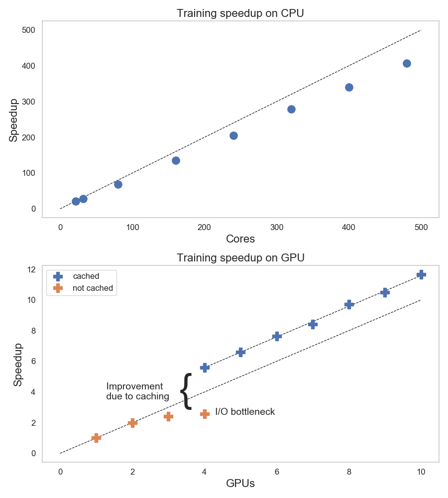
    A useful parameter to study scalability is the "Speedup": if you execute your job with "p" (as in parallel) concurrent processes, Speedup(p) is defined as the response time of the job at concurrency p divided the response time of the job run with p=1. If you prefer a formula: Speedup(p) = R(1)/R(p).
    The expected behavior for the speedup of a perfectly scalable job will show as a straight line in a graph of speedup vs. number of concurrent tasks: the amount of work is directly proportional to the number of workers in this case. Any bottleneck and/or serialization effect will cause the graph of the speedup to eventually "bend down" and lay below the "ideal case" of linear scalability. See also how the speedup can be modeled using Amdahl's law.
    The following table and graph show the measurements of Lab 8 (query execution time for reading the test table of 68 GB) transformed into speedup values vs. N# of executors:

    p=N# executors
    Elapsed time (s)
    Speedup(p)
    1 311302 1.00
    2 149673 2.08
    3 100194 3.11
    4 75547 4.12
    5 60931 5.11
    6 51342 6.06
    7 44165 7.05
    8 39613 7.86
    9 35450 8.78
    10 32061 9.71
    11 29436 10.58
    12 27735 11.22
    13 25764 12.08
    14 24021 12.96
    15 23217 13.41
    16 22092 14.09
    17 21016 14.81
    18 20647 15.08
    19 19999 15.57
    20 19989 15.57


    Lessons learned:
    • The speedup grows almost linearly, at least up to about 10 concurrent tasks
    • This can be interpreted as a sign that the workload scales and does not encounter bottlenecks at least up to the measured scale. 
    • At higher load you can see that the speedup reaches a saturation zone. Drilling down on this is the subject of the next Lab.
     

    Lab 10: CPU utilization, instructions, cycles and memory at scale


    CPU utilization is a metric that does not reveal many insights about the nature of the workload. Measuring CPU instructions and cycles helps in understanding if the workload is instruction-bound or memory-bound. Also measuring the throughput between CPU and memory is important for data-intensive workloads as the one tested here.
    The following graph reports the measurement of the CPU-to-memory throughput for the test workloads measured using Intel's pcm (see also this link for more info).


    CPU-to-memory traffic measurement at high load - Here below some key metrics measured in the test with 20 concurrent tasks executing the test workload:
    • The measured throughput of data transfer between CPU and memory is about 84 GB/s (55% of which is writes and 45% reads). 
    • Another important metric is the utilization of the QPI links, there are 4 links in total in the system (2 links per socket). The measured QPI utilization is ~65% for the test with 20 concurrent processes.

    Comparing with benchmarks - The question I would like to answer is: I have measured 84 GB/s of CPU-to-memory throughput, is that a high value for my test system? To approach the problem I have used a couple of benchmark tools to generate high load on the system: John D. McCalpin's stream memory test and Intel memory latency latency checker, see further details on those tools at this link. The test system during the stress tests has reached up to 100 GB/s of CPU-to-memory throughput with the benchmark tools. By comparing the benchmark values with the measured throughput of 84 GB/s I am tempted to conclude that the test workload (reading a Parquet table) stresses the system towards saturation levels of the CPU-to-memory channel at high load (with 20 cores busy executing tasks).

    IPC measurement under load - Another measure hinting that the CPUs are spending an increasing amount of time in stalled cycles at high load, comes from the measurement of instruction per cycle (IPC). The number of instructions for the test workload (reading 68 GB of a test Parquet table) stays constant at about 1.3E12 instructions at various load levels (this number can be measured with perf for example). However, the number of cycles needed to process the workload increases with load. Measurements on a the test system are reported in the following figure:


    Comments on IPC measurements - By comparing the graph of job speedup and the graph of IPC, you can see that the drop in IPC corresponds to the inflection point in the scalability graph, around a number of concurrent tasks ~10. This is a good hint that serialization mechanism are in place to limit the scalability when the load is higher than 10 concurrent tasks (for the test system used).
    Additional notes on the measurements of IPC at scale:
    - The measurements reported are an average of the IPC values measured over the duration of the job, there is more structure to it when looking at a finer time scale, which is not reported here.
    - The measured amount of data transferred between CPU and memory shows a slow linear increase with number of concurrent tasks (from ~1300 GB at N# tasks=1 to 1.6 TB at N# tasks=20).
       
    Lessons learned: 
    • The test workload in this post (reading a partitioned Parquet table) when run with concurrently executing tasks, scales up linearly to about 10 concurrent tasks, then the scalability appears affected by the higher utilization of the CPU-memory channels. 
    • The highest throughput of the test with Spark SQL measured with 20 concurrent tasks is  ~3.4 GB/s of Parquet data processed and this correspond to ~84 GB/s throughput between CPUs and memory.
    • As noted in Lab 7, to process 68 GB of parquet data in the test workload used in this post, the system has accessed more than 1 TB of memory. Similarly, at high load  the throughput observed at the user-end is of about 3.4 GB/s RAM while the system throughput  at systems level at 84 GB/s. The high ratio of useful work done compared to the system load hints to possible optimizations in the Parquet reader.

    Lab 11: Understanding CPU metrics with hyper-threading and pitfalls when measuring CPU workloads on multi-tenant systems


    In this section I want to drill down on a few pitfalls when measuring CPU utilization. The first one is about CPU Hyper-Threading.
    The server used for the tests reported here has hyper-threading activated. In practice this means that the OS sees "40 CPU" (see for example /proc/cpuinfo), while the actual number of cores in the system is 20. In the previous Labs you have seen how the test workload scales up to 20 concurrent tasks, the number 20 being the number of cores in the system. In that "load regime" the OS appeared to be able to schedule the tasks and utilize the available CPU cores to scale up the workload (the test system was dedicated to the tests and did not have any other relevant load). The following test is about scaling up to 40 concurrent tasks and comparing with the case of 20 concurrent tasks.

    Metric 20 concurrent tasks 40 concurrent tasks
    Elapsed time 20 s 23 s
    Executor run time 392 s 892 s
    Executor CPU Time 376 s 849 s
    CPU-memory data volume 1.6 TB 2.2 TB
    CPU-memory throughput 85 GB/s 90 GB/s
    IPC 1.42 0.66
    QPI utilization 65% 80%


    Lessons learned:


    • The response time of the test workload does not improve when going from 20 concurrent tasks up to 40 concurrent tasks. 
    • The measured SQL elapsed time stays basically constant, actually it increases slightly for the chosen workload. The increase in elapsed time (i.e. a reduction of throughput) can be correlated with the extra work in CPU-to-memory data transfer, that grows with the number of threads utilized by the load (this is also reported in the measurements table).
    • The OS scheduler runs 40 concurrent processes/tasks, corresponding to the number of threads in the CPUs, however this does not improve the performance compared to the case of 20 concurrent processes/tasks.
    • When CPU utilization goes above 20 concurrent processes, some of the processes are scheduled to run on threads that have to share the same physical cores (up to 2 threads per core in the CPU used in the test system). The end result is that the system behaves as if it was running on slower CPUs (roughly twice slower moving from load= 20 concurrent tasks to load=40 concurrent tasks).
    • Gotcha: process utilization and measured CPU time are difficult metrics to interpret and even more so when using hyper-threading, this can be an important point to keep in mind when troubleshooting workloads at high load and/or on multi-tenant systems utilizing shared resources where the additional load can come from other "noisy neighbors".

    In the previous paragraphs you have seen that when the number of concurrent tasks goes above the number of available CPU cores in the system, the throughput of the test workload does not increase, even though the OS reports an increasing utilization of the CPU threads.
    What happens when the number of concurrent tasks keeps increasing and goes above the number of available CPU threads in the system?
    This is another case of running on a system with high load and it is a valid case, possibly because you are running on a system shared with other users creating additional load. Here is an example, when running the workload with 60 concurrent tasks (the test system has 40 CPU threads):

    Metric 20 concurrent tasks 40 concurrent tasks 60 concurrent tasks
    Elapsed time 20 s 23 s 23 s
    Executor run time 392 s 892 s 1354 s
    Executor CPU Time 376 s 849 s 872 s
    CPU-memory data volume 1.6 TB 2.2 TB 2.2 TB
    CPU-memory throughput 85 GB/s 90 GB/s 90 GB/s
    IPC 1.42 0.66 0.63
    QPI utilization 65% 80% 80%

      
    Key points: 
    • At high load the job latency stays constant with increasing load, roughly to the value reached when running with 20 concurrent tasks (that is about 20 seconds, 20 concurrent tasks corresponds to one task per core in the test system).
    • The amount of utilized CPU seconds does not increase above the value measured at 40 concurrent tasks. This is explained as the OS can schedule work on 40 "logical CPUs" corresponding to 40 possible concurrent execution threads in the CPUs using hyper-threading.
    • When the number of concurrent tasks is higher than the number of available CPU threads (40) the measured CPU utilization time does not increase, while the sum of the elapsed time on the executor processes keeps increasing. The additional executor time measured accounts for time spent waiting in OS scheduler queues.
    • Gotcha: The amount of useful work that the system does when executing the test workload at 20, 40 or 60 concurrent tasks is very similar. In all cases the workload is CPU-bound, with high throughput to memory. The measured metrics values CPU time and executor run time can be misleading at high load for the reasons just explained. It is useful to bear in mind this type of examples when troubleshooting workloads on shared/multi-tenant systems, where additional load on the system can come from sources external to your jobs.
      

    Conclusions


    CPU-bound workloads  are very important in data processing. In particular modern hardware has typically abundance of cores and memory. Technologies like Spark, Parquet, Hadoop, make data processing at scale easier and cheaper. Techniques and tools for measuring and understanding data processing workloads, including their CPU and memory footprint, are important to get the best value out of your software and hardware investment.
    Reading from Parquet is a CPU-bound workload examined in this post. Some of the lessons learned investigating the test workloads are:

    • Spark metrics can be used to understand resource usage and workload behavior, with some limitations.
    • Use OS-tools to measure CPU, network, disk. Dynamic tracing can drill down on  latency. Stack profiling and flame graphs are useful to drill down on hot parts of the code
    • CPU utilization does not always give the full picture: use hardware counters to drill down, including instructions and cycles (IPC) and CPU-to-memory throughput. 
    • Measure your workload, speedup, IPC, CPU utilization, as function of increasing number of concurrent tasks to understand its scalability profile and bottlenecks.
    • Watch out for common pitfalls when measuring CPU metrics on multi-tenant systems, in particular be aware if Hyper-threading is used.
      

    Relevant articles and presentations:


    - Brendan Gregg's blog post CPU Utilization is Wrong
    - The presentation: A Crash Course in Modern Hardware by Cliff Click
    Brendan Gregg's page on Flame Graphs
    Nitsan Wakart: Using FlameGraphs To Illuminate The JVM by , Exploring Java Perf Flamegraphs
    - For related topics in the Oracle context, see Tanel Poders's blog post "RAM is the new disk"
    Intel 64 and IA-32 Architectures, Optimization Reference Manual
    Intel Tuning Guides and Performance Analysis Papers


    Acknowledgements

    This  work has been done in the context of CERN Hadoop and Spark service and has profited from the collaboration of several of my colleagues at CERN.