Apache Spark is incredibly powerful, but anyone who has
worked with it long enough knows the feeling:
Why is this job suddenly slower today? Why are executors running out of memory? Why is one stage taking 90% of the runtime? What exactly is Spark doing behind the scenes?
The Spark UI already provides a lot of useful information, but collecting, visualizing, and analyzing performance metrics at scale often requires additional tooling.
Over the years, we have developed and open-sourced a set of complementary tools to help Spark users monitor, troubleshoot, and better understand their workloads from notebooks to production clusters.
In this post, we present the three Spark monitoring tools we publish and actively use at CERN.
Three Different Tools, Three Different Perspectives on
Spark
Each tool addresses a different layer of Spark
observability:
If you use Spark interactively, tune jobs, or benchmark
workloads, chances are you have wished for an easier way to collect performance
metrics directly from your code.
sparkMeasure provides lightweight instrumentation for Apache
Spark applications and exposes metrics directly inside Scala and PySpark
workflows.
Why Users Like It
One major advantage of sparkMeasure is simplicity.
A few lines of code are enough to start collecting
meaningful metrics.
Example Use Cases
Compare
two DataFrame/SQL optimization strategies
Investigate
shuffle-heavy workloads
Measure
the impact of partitioning changes
Capture
metrics during automated tests
Export
performance summaries to DataFrames
Adoption
sparkMeasure has seen strong adoption in the Spark
community. The sparkMeasure's Python wrapper package alone currently (May 2026) exceeds 1 million downloadsper month. This level of usage demonstrates how broadly useful
lightweight Spark instrumentation has become.
Figure 1: Architecture diagram showing how sparkMeasure integrates with the Spark's executors task metrics system to collect, aggregate, and expose Spark execution metrics for analysis and troubleshooting.
2. SparkMonitor — Making Spark Friendlier in Notebooks
SparkMonitor was originally developed for CERN’s hosted
notebook environments to improve the Spark experience for users running Jupyter
notebooks interactively.
It provides notebook-friendly monitoring and visualization
capabilities that make Spark behavior easier to understand while jobs are
running.
The goal is simple:
Make Spark execution more transparent and easier to follow
directly from the notebook environment.
Figure 2: Animated view of sparkmonitor in action, showing Spark job progress and helping users visualize execution flow, resource usage, and runtime behavior directly from the notebook environment.
3. Spark Dashboard — Real-Time Observability for Spark
Clusters
Real-time dashboards help answer operational questions such
as:
Are
executors under memory pressure or CPU bound or I/O bound?
Is the
cluster saturated?
Did a
deployment introduce regressions?
At CERN, this dashboard is also used internally as an optional enhanced monitoring solution for Spark services.
The added value:
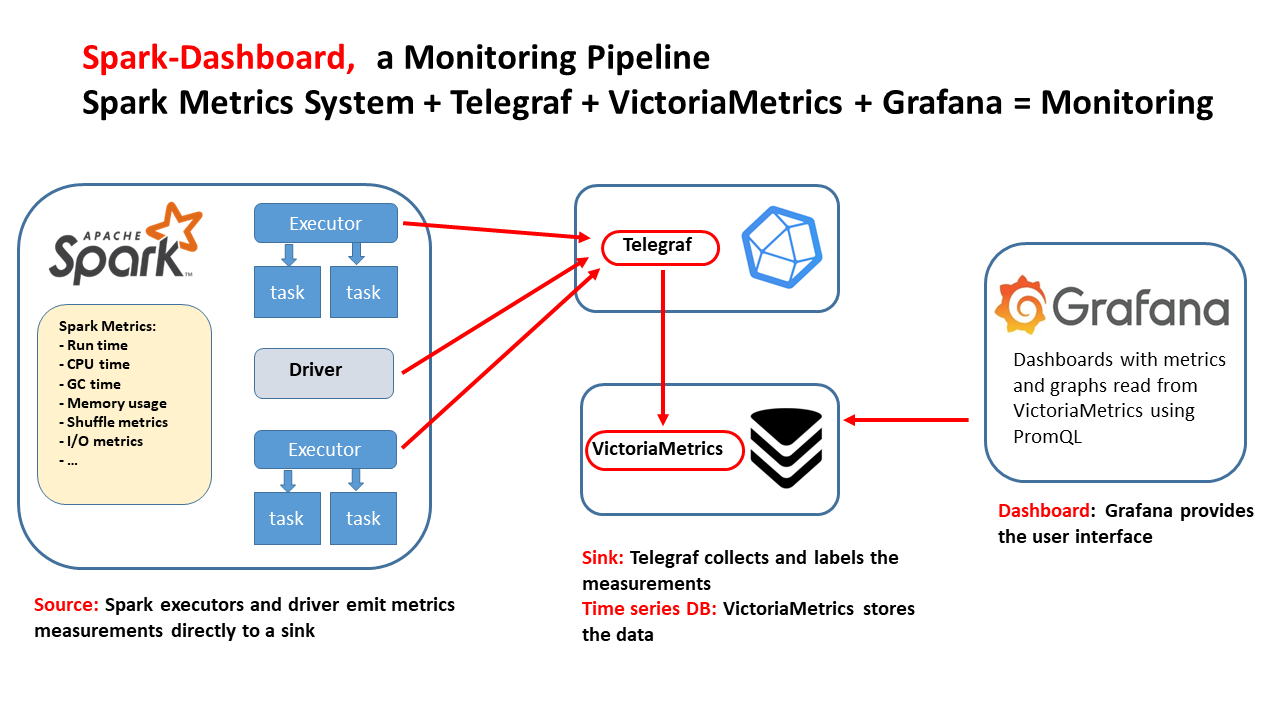
The goal of Spark Dashboard is to provide a ready-to-use real-time monitoring stack for Spark, packaged as Docker images and Helm charts, with integrations already configured for Telegraf, VictoriaMetrics, and Grafana dashboards.
This makes it easy to deploy end-to-end Spark observability, from a laptop to large Kubernetes clusters.
Figure 3: Architecture of the Spark Dashboard monitoring stack, integrating Spark metrics (via the Dropwizard Metrics library) with time-series collection and storage using Telegraf and VictoriaMetrics, and real-time visualization through Grafana dashboards.
Test-Driving the Monitoring Tools with TPC-DS Benchmarks
A practical way to explore and validate these monitoring
tools is to run them against reproducible Spark benchmark workloads such as
TPC-DS.
We use an open-source PySpark wrapper for TPC-DS benchmark
execution: TPCDS PySpark Wrapper
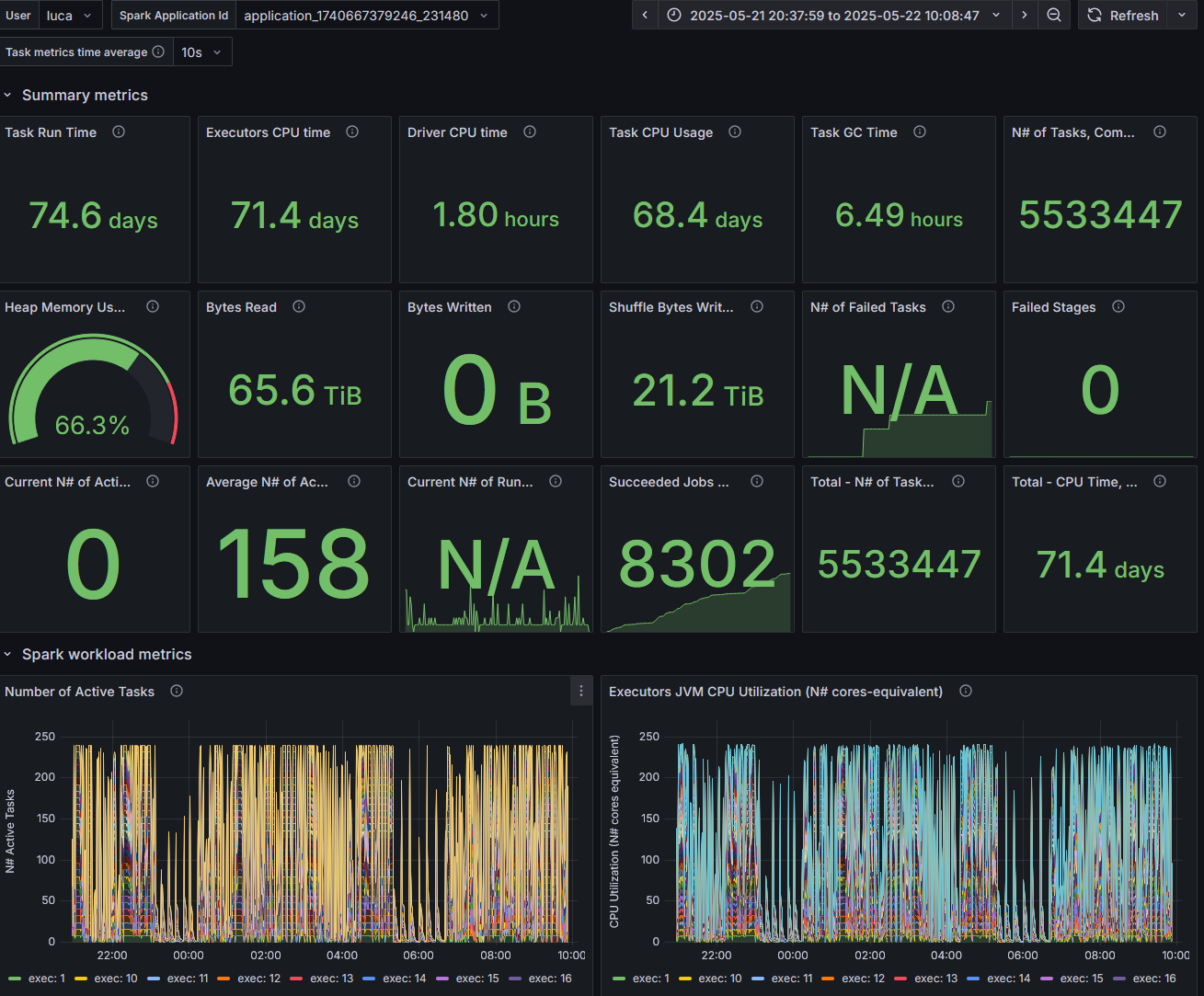
Figure 4: Snapshot from the Spark Dashboard captured during the execution of the TPC-DS benchmark at 10 TB scale, illustrating real-time cluster activity and Spark resource utilization.
Complementary Rather Than Competing
These tools are designed to work at different levels. Think of them as complementary building blocks.
Open Source and Community
All three projects are open source and publicly available on
GitHub.
Spark applications can sometimes feel like black boxes.
The more visibility users have into execution behavior,
metrics, and resource consumption, the easier it becomes to:
optimize
workloads,
troubleshoot
issues,
improve
cluster efficiency,
and
teach others how Spark really works.
We hope these tools help make Spark more observable,
understandable, and easier to operate, whether you are running a single
notebook or a large production platform.
If you are already using them, we would love to hear about
your use cases and feedback from the community.
Acknowledgements
This work builds on the contributions of the CERN Databases and Data Analytics group, whose expertise and support have been instrumental in developing and operating the Hadoop, SWAN, and Spark services on which these tools and experiments rely.
TL;DR: Apache Spark 4 lets you build first-class data sources in pure Python. If your reader yields Arrow RecordBatch objects, Spark ingests them with reduced Python↔JVM serialization overhead. I used this to ship a ROOT data format reader for PySpark.
A PySpark reader for the ROOT format
ROOT is the de-facto data format across High-Energy Physics; CERN experiments alone store over an exabytes of data in ROOT files. With Spark 4’s Python API, building a ROOT reader becomes a focused Python exercise: parse with Uproot/Awkward, produce a PyArrow Table, yield RecordBatch, and let Spark do the rest.
Yield arrow batches, skip the row-by-row serialization tax
Spark 4 introduces a Python data source that makes it simple to ingest data via Python libraries. The basic version yields Python rows (incurring per-row Python↔JVM hops). With direct Arrow batch support (SPARK-48493) your DataSourceReader.read() can yield pyarrow.RecordBatch objects so Spark ingests columnar data in batches, dramatically reducing cross-boundary overhead.
ROOT → Arrow → Spark in a few moving parts
Here’s the essence of the ROOT data format reader I implemented and packaged in pyspark-root-datasource:
Subclass the DataSource and DataSourceReader from pyspark.sql.datasource.
In read(partition), produce pyarrow.RecordBatch objects.
Register your source with spark.dataSource.register(...), then spark.read.format("root")....
Minimal, schematic code (pared down for clarity):
from pyspark.sql.datasource import DataSource, DataSourceReader, InputPartition

class RootDataSource(DataSource):
    @classmethod
    def name(cls):
        return "root"
    def schema(self):
        # Return a Spark schema (string or StructType) or infer in the reader.
        return "nMuon int, Muon_pt array<float>, Muon_eta array<float>"
    def reader(self, schema):
        return RootReader(schema, self.options)

class RootReader(DataSourceReader):
    def __init__(self, schema, options):
        self.schema = schema
        self.path = options.get("path")
        self.tree = options.get("tree", "Events")
        self.step_size = int(options.get("step_size", 1_000_000))

    def partitions(self):
        # Example: split work into N partitions
        N = 8
        return [InputPartition(i) for i in range(N)]

    def read(self, partition):
        import uproot, awkward as ak
        start = partition.index * self.step_size
        stop  = start + self.step_size
        with uproot.open(self.path) as f:
            arrays = f[self.tree].arrays(entry_start=start, entry_stop=stop, how=ak.Array)
        table = ak.to_arrow_table(arrays, list_to32=True)
        for batch in table.to_batches():   # <-- yield Arrow RecordBatches directly
            yield batch
Why this felt easy
Tiny surface area: one DataSource, one DataSourceReader, and a read() generator. The Spark docs walk through the exact hooks and options: Apache Spark
Python-native stack: I could leverage existing Python libraries for reading the ROOT format and for processing Arrow, Uproot + Awkward + PyArrow, with no additional Scala/Java code.
Arrow batches = speed: SPARK-48493 wires Arrow batches into the reader path to avoid per-row conversion. issues.apache.org
Practical tips
Provide a schema if you can. It enables early pruning and tighter I/O; the Spark guide covers schema handling and type conversions.
Partitioning matters. ROOT TTrees can be large and jagged: tune step_size to balance task parallelism and batch size. (The reader exposes options for this.)
Arrow knobs. For very large datasets, controlling Arrow batch sizes can improve downstream pipeline behavior; see Spark’s Arrow notes.
“Show me the full thing”
If you want a working reader with options for local files, directories, globs, and the XRootD protocol (root://), check out the package at: pyspark-root-datasource
Apache Spark is renowned for its speed and efficiency in handling large-scale data processing. However, optimizing Spark to achieve maximum performance requires a precise understanding of its inner workings. This blog post will guide you through establishing a Spark Performance Lab with essential tools and techniques aimed at enhancing Spark performance through detailed metrics analysis.
Why a Spark Performance Lab
The purpose of a Spark Performance Lab isn't just to measure the elapsed time of your Spark jobs but to understand the underlying performance metrics deeply. By using these metrics, you can create models that explain what's happening within Spark's execution and identify areas for improvement. Here are some key reasons to set up a Spark Performance Lab:
Hands-on learning and testing: A controlled lab setting allows for safer experimentation with Spark configurations and tuning and also experimenting and understanding the monitoring tools and Spark-generated metrics.
Load and scale: Our lab uses a workload generator, running TPCDS queries. This is a well-known set of complex queries that is representative of OLAP workloads, and that can easily be scaled up for testing from GBs to 100s of TBs.
Improving your toolkit: Having a toolbox is invaluable, however you need to practice and understand their output in a sandbox environment before moving to production.
Get value from the Spark metric system: Instead of focusing solely on how long a job takes, use detailed metrics to understand the performance and spot inefficiencies.
Tools and Components
In our Spark Performance Lab, several key tools and components form the backbone of our testing and monitoring environment:
Workload generator:
We use a custom tool, TPCDS-PySpark, to generate a consistent set of queries (TPCDS benchmark), creating a reliable testing framework.
Spark instrumentation:
Spark’s built-in Web UIfor initial metrics and job visualization.
Custom tools:
SparkMeasure: Use this for detailed performance metrics collection.
Spark-Dashboard: Use this to monitor Spark jobs and visualize key performance metrics.
Additional tools for Performance Measurement include:
These quick demos and tutorials will show you how to use the tools in this Spark Performance Lab. You can follow along and get the same results on your own, which will help you start learning and exploring.
Figure 1: The graph illustrates the dynamic task allocation in a Spark application during a TPCDS 10TB benchmark on a YARN cluster with 256 cores. It showcases the variability in the number of active tasks over time, highlighting instances of execution "long tails" and straggler tasks, as seen in the periodic spikes and troughs.
How to Make the Best of Spark Metrics System
Understanding and utilizing Spark's metrics system is crucial for optimization:
Importance of Metrics: Metrics provide insights beyond simple timing, revealing details about task execution, resource utilization, and bottlenecks.
Execution Time is Not Enough: Measuring the execution time of a job (how long it took to run it), is useful, but it doesn’t show the whole picture. Say the job ran in 10 seconds. It's crucial to understand why it took 10 seconds instead of 100 seconds or just 1 second. What was slowing things down? Was it the CPU, data input/output, or something else, like data shuffling? This helps us identify the root causes of performance issues.
Key Metrics to Collect:
Executor Run Time: Total time executors spend processing tasks.
Executor CPU Time: Direct CPU time consumed by tasks.
JVM GC Time: Time spent in garbage collection, affecting performance.
Shuffle and I/O Metrics: Critical for understanding data movement and disk interactions.
Memory Metrics: Key for performance and troubleshooting Out Of Memory errors.
Metrics Analysis, what to look for:
Look for bottlenecks: are there resources that are the bottleneck? Are the jobs running mostly on CPU or waiting for I/O or spending a lot of time on Garbage Collection?
USE method: Utilization Saturation and Errors (USE) Method is a methodology for analyzing the performance of any system.
The tools described here can help you to measure and understand Utilization and Saturation.
Can your job use a significant fraction of the available CPU cores?
Examine the measurement of the actual number of active tasks vs. time.
Figure 1 shows the number of active tasks measured while running TPCDS 10TB on a YARN cluster, with 256 cores allocated. The graph shows spikes and troughs.
Understand the root causes of the troughs using metrics and monitoring data. The reasons can be many: resource allocation, partition skew, straggler tasks, stage boundaries, etc.
Which tool should I use?
Start with using the Spark Web UI
Instrument your jobs with sparkMesure. This is recommended early in the application development, testing, and for Continuous Integration (CI) pipelines.
Observe your Spark application execution profile with Spark-Dashboard.
Use available tools with OS metrics too. See also Spark-Dashboard extended instrumentation: it collects and visualizes OS metrics (from cgroup statistics) like network stats, etc
For those interested in delving deeper into Spark instrumentation and metrics, the Spark documentation offers a comprehensive guide.
SparkMeasure: This tool captures metrics directly from Spark’s instrumentation via the Listener Bus. For a detailed understanding of how it operates, refer to the SparkMeasure architecture. It specifically gathers data from Spark's Task Metrics System, which you can explore further here.
Figure 2: This technical drawing outlines the integrated monitoring pipeline for Apache Spark implemented by Spark-Dashboard using open-source components. The flow of the diagram illustrates the Spark metrics source and the components used to store and visualize the metrics.
Lessons Learned and Conclusions
From setting up and running a Spark Performance Lab, here are some key takeaways:
Collect, analyze and visualize metrics: Go beyond just measuring jobs' execution times to troubleshoot and fine-tune Spark performance effectively.
Use the Right Tools: Familiarize yourself with tools for performance measurement and monitoring.
Start Small, Scale Up: Begin with smaller datasets and configurations, then gradually scale to test larger, more complex scenarios.
Tuning is an Iterative Process: Experiment with different configurations, parallelism levels, and data partitioning strategies to find the best setup for your workload.
Establishing a Spark Performance Lab is a fundamental step for any data engineer aiming to master Spark's performance aspects. By integrating tools like Web UI, TPCDS_PySpark, sparkMeasure, and Spark-Dashboard, developers and data engineers can gain unprecedented insights into Spark operations and optimizations.
Explore this lab setup to turn theory into expertise in managing and optimizing Apache Spark. Learn by doing and experimentation!
Acknowledgements: A special acknowledgment goes out to the teams behind the CERN data
analytics, monitoring, and web notebook services, as well as the
dedicated members of the ATLAS database group.
Resources
To get started with the tools mentioned in this blog:
TL;DR Explore a step-by-step example of troubleshooting Apache Spark job performance using flame graph visualization and profiling. Discover the seamless integration of Grafana Pyroscope with Spark for streamlined data collection and visualization.
The Puzzle of the Slow Query
Set within the framework of data analysis for the ATLAS experiment's Data Control System, our exploration uses data stored in the Parquet format and deploys Apache Spark for queries. The setup: Jupyter notebooks operating on the SWAN service at CERN interfacing with the Hadoop and Spark service.
The Hiccup: A notably slow query during data analysis where two tables are joined. Running on 32 cores, this query takes 27 minutes—surprisingly long given the amount of data in play.
The tables involved:
EVENTHISTORY: A log of events for specific sub-detectors, each row contains a timestamp, the subsystem id and a value
EVENTHISTORY is a large table, it can collect millions of data points per day, while LUMINOSITY is a much smaller table (only thousands of points per day). In the test case reported here we used data collected over 1 day, with EVENTHISTORY -> 75M records, and LUMINOSITY -> 2K records.
The join condition between EVENTHISTORY and LUMINOSITY is an expression used to match for events in EVENTHISORY and intervals in LUMINOSITY (note this is not a join based on an equality predicate). This is what the query looks like in SQL:
An alternative version of the same query written using the DataFrame API:
eventhistory_df.join(
luminosity_df,
(eventhistory_df.ts >= luminosity_df.starttime) &
(eventhistory_df.ts <= luminosity_df.endtime)
).select(luminosity_df.LUMI_NUMBER,
eventhistory_df.ELEMENT_ID,
eventhistory_df.VALUE_NUMBER)
Cracking the Performance Case
WebUI: The first point of entry for troubleshooting this was the Spark WebUI. We could find there the execution time of the query (27 minutes) and details on the execution plan and SQL metrics under the "SQL/ DataFrame" tab. Figure 1 shows a relevant snippet where we could clearly see that Broadcast nested loop join was used for this.
Execution Plan: The execution plan is the one we wanted for this query, that is the small LUMINOSITY table is broadcasted to all the executors and then joined with each partition of the larger EVENTHISTORY table.
Figure 1: This shows a relevant snippet of the execution graph from the Spark WebUI. The slow query discussed in this post runs using broadcast nested loops join. This means that the small table is broadcasted to all the nodes and then joined to each partition of the larger table.
CPU utilization measured with Spark Dashboard
Spark Dashboard instrumentation provides a way to collect and visualize Spark execution metrics. This makes it easy to plot the CPU used during the SQL execution. From there we could see that the workload was CPU-bound
The Clue: Profiling with Flame Graphs and Pyroscope
Stack profiling and Flame Graphs visualization are powerful techniques to investigate CPU-bound workloads. We use it here to find where the CPU cycles are consumed and thus make the query slow.
First a little recap of what is stack profiling with flame graph visualization, and what tools we can use to apply it to Apache Spark workloads:
Stack profiling and Flame Graphs visualization provide a powerful technique for troubleshooting CPU-bound workloads.
Flame Graphs provide information on the "hot methods" consuming CPU
Flame Graphs and profiling can also be used to profile time spent waiting (off-cpu) and memory allocation
Grafana Pyroscopesimplifies data collections and visualization, using agents and a custom WebUI. Key motivations for using it with Spark are:
Streamlined Data Collection & Visualization: The Pyroscope project page
offers a simplified approach to data gathering and visualization with its custom WebUI and agent integration.
Java Integration: The Pyroscope java agent
is tailored to work seamlessly with Spark. This integration shines especially when Spark is running on various
clusters such as YARN, K8S, or standalone Spark clusters.
Correlation with Grafana: Grafana’s integration with Pyroscope lets you juxtapose metrics with other
instruments, including the Spark metrics dashboard.
Proven Underlying Technology: For Java and Python, the tech essentials for collecting stack profiling data,
async-profiler and py-spy,
are time-tested and reliable.
Functional & Detailed WebUI: Pyroscope’s WebUI stands out with features that allow users to:
Select specific data periods
Store and display data across various measurements
Offer functionalities to contrast and differentiate measurements
Showcase collected data for all Spark executors, with an option to focus on individual executors or machines
Lightweight Data Acquisition: The Pyroscope java agent is efficient in data gathering. By default, stacks are sampled every 10 milliseconds and uploaded every 10 seconds. We did not observe any measurable performance or stability impact of the instrumentation.
Spark Configuration
To use Pyroscope with Spark we used some additional configurations. Note this uses a specialized Spark Plugin from this repo. It is also possible to use java agents. The details are at:
Figure 2: This is a snapshot from the Grafana Pyroscope dashboard with data collected during the execution of the slow query (join between EVENTHISTORY and LUMINOSITY). The query runs in 27 minutes, using 32 cores. The Flame Graph shows the top executed methods and the Flame Graph. Notably, a large fraction of the execution time appears to be spent into SparkDateTimeUtils performing date-datatype conversion operations. This is a crucial finding for the rest of the troubleshooting and proposed fix.
The Insight
Using profiling data from Pyroscope, we pinpointed the root cause of the query's sluggishness. Spark was expending excessive CPU cycles on data type conversion operations during the evaluation of the join predicate. Upon revisiting the WebUI and delving deeper into the execution plan under the SQL/DataFrame tab, we discovered, almost concealed in plain view, the specific step responsible for the heightened CPU consumption:
(9) BroadcastNestedLoopJoin [codegen id : 2]
Join condition: ((ts#1 >= cast(starttime_dec#57 as timestamp)) AND (ts#1 <= cast(endtime_dec#58 as timestamp)))
The extra operations of "cast to timestamp" appear to be key in explaining the issue.
Why do we have date format conversions?
By inspecting the schema of the involved tables, it turns out that in the LUMINOSITY table the fields used for joining with the timestamp are of type Decimal.
To recap, profiling data, together with the execution plan, showed that the query was slow because it forced data type conversion over and over for each row where the join condition was evaluated.
The fix:
The solution we applied for this was simple: we converted to use the same data type for all the columns involved in the join, in particular converting to timestamp the columns starttime and endtime of the LUMINOSITY table.
Results: improved performance 70x:
The results are that the query after the change runs in 23 sec, compared to the previous runtime of 27 minutes. Figure 3 shows the Flame graph after the fix was applied.
Figure 3: This is a snapshot of the Grafana Pyroscope dashboard with data collected during the execution of the query after tuning. The query takes only 23 seconds compared to 27 minutes before tuning (see Figure 2)
Related work and links
Details of how to use Pyroscope with Spark can be found in the note:
Related work of interest for Apache Spark performance troubleshooting:
Spark Dashboard - tooling and configuration for deploying an Apache Spark Performance Dashboard using containers technology.
Spark Measure - a tool for performance troubleshooting of Apache Spark workloads. It
simplifies the collection and analysis of Spark task and stage metrics
data.
Spark Plugins - Code and examples of how to write and deploy Apache Spark Plugins.
Wrapping Up: Stack profiling and Flame Graph visualization aren’t just jargon—they’re game-changers. Our deep dive illuminated how they transformed an Apache Spark query performance by 70x. Using Grafana Pyroscope with Spark, we demonstrated a holistic approach to gather, analyze, and leverage stack profile data.
A hearty thank you to my colleagues at CERN for their guidance. A special nod to the CERN data analytics, monitoring, and web notebook services, and to the ATLAS database team.
Dive into a comprehensive load-testing exploration using Apache Spark with CPU-intensive workloads. This blog provides a comparative analysis of five distinct JDKs' performance under heavy-duty tasks generated through Spark. Discover a meticulous breakdown of our testing methodology, tools, and insightful results. Keep in mind, our observations primarily indicate the test toolkit and system's performance rather than offering a broad evaluation of the JDKs.
In this post, we'll also emphasize:
The rationale behind focusing on CPU and memory-intensive workloads, especially when handling large Parquet datasets.
The load testing tool's design: stressing CPU and memory bandwidth with large Parquet files.
Key findings from our tests, offering insights into variations across different JDKs.
Tools and methods employed for the most accurate measurements, ensuring our results are as reflective of real-world scenarios as possible.
Join us on this journey to decipher the intricate landscape of JDKs in the realm of Apache Spark performance!
On the load testing tool and instrumentation
What is being measured:
this is a microbenchmark of CPU and memory bandwidth, the tool is not intended to measure the performance of Spark SQL.
this follows the general ideas of active benchmarking: a load generator is used to produce CPU and memory-intensive load,
while the load is measured with instrumentation.
Why testing with a CPU and memory-intensive workload:
In real life, the CPU and memory intensive workloads are often the most critical ones. In particular, when working with
large datasets in Parquet format, the CPU and memory-intensive workloads are often the most critical ones.
Moreover, workloads that include I/O time from object storage can introduce a lot of variability in the results that
does not reflect the performance of Apache Spark but rather of the object storage system.
Working on a single large machine also reduces the variability of the results and makes it easier to compare the
performance of different test configurations.
The test kit:
The testing toolkit used for this exercise is described at test_Spark_CPU_memory.
The tool generates CPU and memory-intensive load, with a configurable number of concurrent workers.
It works by reading a large Parquet file. The test setup is such that the file is cached in the system memory
therefore the tool mostly stresses CPU and memory bandwidth.
Instrumentation:
The workload is mostly CPU-bound, therefore the main metrics of interest are CPU time and elapsed time.
Using sparkMeasure, we can also collect metrics on the Spark executors, notably the executors' cumulative elapsed time,
CPU time, and time in garbage collection.
Workload data:
The test data used to generate the workload is a large Parquet table, store_sales, taken from the open source TPCDS benchmark.
The size of the test data is 200 GB, and it is stored in multiple Parquet files. You can also use a subset of the files in case you want to scale down the benchmark.
The files are cached in the filesystem cache, so that the test kit mostly stresses CPU and memory bandwidth (note,
this requires 512GB of RAM on the test system, if you have less RAM, reduce the dataset size).
Test results:
Tests were run using the script spark_test_JDKs.sh that runs test_Spark_CPU_memory.py
with different JDKs and prints out the results.
The output of three different tests were collected and stored in txt files that can be found in the Data folder.
Test system:
A server with dual CPUS (AMD Zen 2 architecture), 16 physical cores each, 512 GB RAM, ~300 GB of storage space.
Spark configuration:
We use Apache Spark run in local mode (that is on a single machine, not scaling out on a cluster) for these tests,
with 64GB of heap memory and 20 cores allocated to Spark.
The large heap memory allocation is to reduce Garbage Collection overhead, which still fits in the available RAM.
The number of cores for Spark (that is the maximum number of concurrent tasks being executed by Spark) is set to 20,
which brings the CPU load during the test execution to use about 60% of the physical cores, the workload keeps the
CPUs busy with processing Parquet files, the rest of the CPU power is available for running other accessory load, notably
Garbage collection activities, the OS and other processes.
Example performance test results:
This shows how you can use the toolkit to run the performance tests and collect performance measurements:
$ export JAVA_HOME=.... # Set the JDK that will be used by Spark
$ ./test_Spark_CPU_memory.py --num_workers 20 # Run the 3 tests using 20 concurrent workers (Spark cores)

Allocating a Spark session in local mode with 20 concurrent tasks
Heap memory size = 64g, data_path = ./store_sales.parquet
sparkmeasure_path = spark-measure_2.12-0.23.jar
Scheduling job number 1
Job finished, job_run_time (elapsed time) = 43.93 sec
...executors Run Time = 843.76 sec
...executors CPU Time = 800.18 sec
...executors jvmGC Time = 27.43 sec
Scheduling job number 2
Job finished, job_run_time (elapsed time) = 39.13 sec
...executors Run Time = 770.83 sec
...executors CPU Time = 755.55 sec
...executors jvmGC Time = 14.93 sec
Scheduling job number 3
Job finished, job_run_time (elapsed time) = 38.82 sec
...executors Run Time = 765.22 sec
...executors CPU Time = 751.68 sec
...executors jvmGC Time = 13.32 sec
Notes:
The elapsed time and the Run time decrease with each test run, in
particular from the first to the second run we see a noticeable
improvement,
this is because various internal Spark structures are being "warmed up"
and cached.
In all cases, data is read from the Filesystem cache, except for the
first warm-up runs that are discarded.
Therefore, the test kit mostly stresses CPU and memory bandwidth.
For the test results and comparisons, we will use the values measured at
the 3rd run of each test and average over the
available test results for each category.
JDK comparison tests
The following tests compare the performance of 5 different JDKs, running on Linux (CentOS 7.9),
on a server with dual Zen 2 CPUs, 16 physical cores each, 512 GB RAM, 300 GB of storage space for the test data.
The Apache Spark version is 3.5.0 the test kit is test_Spark_CPU_memory.py.
The JDK tested are:
Adoptium jdk8u392-b08
Adoptium jdk-11.0.21+9
Adoptium jdk-17.0.9+9
Oracle jdk-17.0.9
Oracle graalvm-jdk-17.0.9+11.1
The openJDKs were downloaded from Adoptium Temurin JDK,
the Oracle JDKs were downloaded from Oracle JDK.
The Adoptium Temurin OpenJDK are free to use (see website).
Notably, the Oracle download page also reports that the JDK binaries are available at no cost
under the Oracle No-Fee Terms and Conditions, and the GraalVM Free Terms and Conditions, respectively,
see Oracle's webpage for details.
Test results and measurements
Test results summarized in this table are from the test output files, see Data.
The values reported here are taken from the test reports, measured at
the 3rd run of each test, as the run time improves when running
the tests a couple of times in a row (as internal structures and caches
are warming up, for example), The results are further averaged over the
available test results (6 test runs) and reported for each category.
JDK and Metric name
OpenJDK Java 8
OpenJDK Java 11
OpenJDK Java 17
Oracle Java 17
GraalVM Java 17
JDK
Adoptium jdk8u392-b08
Adoptium jdk-11.0.21+9
Adoptium jdk-11.0.21+9
Oracle jdk-17.0.9
Oracle graalvm-jdk-17.0.9+11.1
Elapsed time (sec)
45.4
39.3
42.0
41.9
34.1
Executors' cumulative ... run time (sec)
896.1
775.9
829.7
828.6
672.3
... CPU time (sec)
851.9
763.4
800.6
796.4
649.5
... Garbage Collection time (sec)
42.6
12.3
29.4
32.5
23.0
Performance data analysis
From the metrics and elapsed time measurements reported above, the key findings are:
Java 8 has the slowest elapsed time, Java 11 and 17 are about 10% faster than Java 8, GraalVM is about 25% faster than Java 8.
The workload is CPU bound.
The instrumentation metrics provide additional clues on understanding the workload and its performance:
Run time, reports the cumulative elapsed time for the executors
CPU time reports the cumulative time spent on CPU.
Garbage Collection Time is the time spent by the executors on JVM Garbage collection, and it is a subset of the "Run time" metric.
From the measured values (see table above) we can conclude that the
executors spend most of the time running tasks "on CPU", with some time
spent on Garbage collection
We can see some fluctuations on Garbage Collection time, with Java 8
having the longest GC time. Note that the algorithm G1GC was used in
all the tests (its use is set
We can see the GraalVM 17 stands out as having the shortest Executors' runtime. We can speculate that is due to the GraalVM
just-in-time compiler and the Native Image feature,
which provide several optimizations compared to the standard HotSpot JVM
(note, before running to install GraalVM for your Spark jobs, please
note that there are other factors
at play here, including that Native Image feature in an optional early
adopter technology, see Oracle documentation for details).
Java 8 shows the worst performance in terms of run time and CPU
time, and it also has the longest Garbage Collection time. This is not
surprising as Java 8 is the oldest
of the JDKs tested here, and it is known to have worse performance than
newer JDKs.
Java 11 and Java 17 have similar performance, with Java 11 being a bit
faster than Java 17 (of the order of 3% for this workload), at this
stage it is not clear if there
is a fundamental reason for this or the difference comes from
measurement noise (see also the section on "sanity checks" and the
comments there on errors in the metrics measurements).
Active benchmarking and sanity checks
The key idea of active benchmarking is that while the load
testing tool is running, we also take several measurements and metrics
using a variety of
monitoring and measuring tools, for OS metrics and application-specific
metrics. These measurements are used to complement the analysis results,
provide sanity checks, and in general to help understand the performance
of the system under test (why is the performance that we see what it
is? why not higher/lower?
Are there any bottlenecks or other issues/errors limiting the
performance?).
Spark tools: the application-specific instrumentation used for these tests were the Spark WebUI and the instrumentation with sparkMeasure
that allowed us to understand the workload as CPU-bound and to measure the CPU time and Garbage collection time.
Java FlameGraph: Link to a FlameGraph of the execution profile taken
during a test run of test_Spark_CPU_memory.py.
The FlameGraph shows that the workload is CPU-bound, and that the time
is spent in the Spark SQL code, in particular in the Parquet reader.
FlameGraphs are a visualization tool for profiling the performance of
applications, see also Tools_FlameGraphs.md.
OS Tools: (see also OS monitoring tools):
Another important aspect was to ensure that the data was cached in the
filesystem cache, to avoid the overhead of reading from disk,
for this tools like iostat and iotop were used to monitor the disk activity and ensure that the I/O on the system was minimal,
therefore implying that data was read from the filesystem cache.
A more direct measurement was taken using cachestat, a tool that can be found in the perf-tools collection and bcc-tool,
which allows measuring how many reads hit the filesystem cache, we could see that the hit rate was 100%,
after the first couple of runs that populated the cache (and that were not taken in consideration for the test results).
CPU measurements were taken using top, htop, and vmstat to monitor the CPU usage and ensure that the CPUs were not saturated.
Other sanity checks: were about checking that the intended JDK was used in a given test, for that we used top and jps, for example.
Another important check is about the stability of the performance tests'
measurements.
We notice fluctuations in the execution time for different runs with the
same parameters, for example.
For this reason the load-testing tool is run on a local machine rather
than a cluster, where these differences are amplified, moreover the
tests are run multiple times,
and the results reported are averages. We estimated the errors in the
metrics measurements due to these fluctuations to be less than 3%, see
also the raw test results reported
available at Data.
Related work
The following references provide additional information on the topics covered in this note.
This blog post presents an exploration of load methodologies using Apache Spark and a custom CPU and memory-intensive testing toolkit. The focus is on comparing different JDKs and producing insights into their respective performance when running Apache Spark jobs under specific conditions (CPU and memory-intensive load when reading Parquet files). Upon evaluating Apache Spark's performance across different JDKs in CPU and memory-intensive tasks involving Parquet files, several key findings emerged:
JDK's Impact: The chosen JDK affects performance, with significant differences observed among Java 8, 11, 17, and GraalVM.
Evolution of JDKs: Newer JDK versions like Java 11 and 17 showcased better outcomes compared to Java 8. GraalVM, with its specific optimizations, also stood out.
Developer Insights: Beyond personal preference, JDK selection can drive performance optimization. Regular software updates are essential.
Limitations: Our results are based on specific test conditions. Real-world scenarios might differ, emphasizing the need for continuous benchmarking.
Guidance for System Specialists: This study offers actionable insights for architects and administrators to enhance system configurations for Spark tasks.
In essence, the choice of JDK, coupled with the nature of the workload, plays a significant role in Apache Spark's efficiency. Continuous assessment is crucial to maintain optimal performance.
Acknowledgements
I would like to express my sincere gratitude to my
colleagues at CERN for their invaluable assistance and insightful
suggestions,
in particular I'd like to acknowledge the CERN data analytics and web
notebook services, and the ATLAS database and data engineering teams.
Introduction to Apache Spark APIs for Data Processing
This is a self-paced and open introduction course to Apache Spark. Theory and demos cover the main Spark APIs:
DataFrame API, Spark SQL, Streaming, Machine Learning. You will also learn how
to deploy Spark on CERN computing resources, notably using the CERN SWAN service. Most tutorials and
exercises are in Python and run on Jupyter notebooks.
Apache Spark is a popular engine for
data processing at scale. Spark provides an expressive API and a scalable
engine that integrates very well with the Hadoop ecosystem as well as with
Cloud resources. Spark is currently used by several projects at CERN, notably
by IT monitoring, by the security team, by the BE NXCALS project, by teams in
ATLAS and CMS. Moreover, Spark is integrated with the CERN Hadoop service, the
CERN Cloud service, and the CERN SWAN web notebooks service.

 Watch sparkMeasure's getting started demo and tutorial