Flame Graphs for Oracle

Topic: This post is a hands-on introduction to using on-CPU Flame Graphs for investigating Oracle workloads. This technique is about collecting and visualizing sampled stack trace data to analyze and troubleshoot Oracle processes at the OS level (in particular applied to Linux).

Motivations: The techniques and tools described here can be used for performance investigations to complement wait-event based information gathered from the Oracle engine, such as information available with ASH and sql monitoring. They can also be used for complex troubleshooting when the wait interface is failing to instrument a particular problem under study. Last but not least they can be used as a learning aid to investigating Oracle internals.

Context and credits: The use of stack sampling has previously been covered for Oracle investigations by Tanel Poder in several articles (see Tanel's Advanced Oracle Troubleshooting Guide and for example this article).
Brendan Gregg has done original work on the collection and visualization of stack sampled data and by introducing the Flame Graphs visualization technique.
The techniques discussed in this post rely on perf for data collection. Perf is a relatively new addition to the performance tools available for Linux (requires kernel 2.6.31 or higher, for example RHEL6 or OL6). A few additional references on using perf for investigating Oracle are: Frits Hoogland, Kevin Closson, Craig Shallahamer.

This article: In this post we will approach the use of stack sampling with perf and visualization with Flame Graphs by introducing examples of growing complexities and by detailing the steps needed to reproduce the results. The main idea is to give a few hints of what this type of approach can do to help us analyze process execution and performance rather than producing a comprehensive guide.

Example 1: Flame Graph of query execution

In Figure 1 here below we can see a Flame Graph representation of the stack traces collected during the execution of "select count(*) from dba_source" (the details of how the graph was generated are described later in this article).

Figure 1: Flame Graph of "select count(*) from dba_source". See more details for each stack layer by hovering over the graph lines in the SVG version

The stack traces expose the name of many Oracle's internal functions. There is no public documentation of those internal functions, however much can be guessed by their name and from the documentation in the Oracle Support document "ORA-600 Lookup Error Categories" (formerly MOS note 175982.1, more recently found as an attachment to Note 1321720.1 and also in other links on the internet).
In addition to the support note, Tanel Poder has already done a great job of "decoding" an important class of internal functions, the rowsource functions with prefix qer (query execution rowsource) in his os_explain script. Rowsource functions expose execution plan details, similarly to what is exposed in ASH data (v$active_session_history) at the columns SQL_PLAN_OPERATION and SQL_PLAN_OPTIONS.
Note also that in Flame Graphs the horizontal axis is not time, stack traces are simply pasted by ordering alphabetically (follow this link to Brendan Gregg's article on Flame Graphs).

If we extract only the rowsource entries from the stack trace data represented in Figure 1, we obtain a simplified Flame Graph, which highlights the parts related to query's execution plan: Figure 2. We can recognize there the execution plan operations and how they stack and nest on top of each other. Although SQL is mainly a declarative language here we have a good view of how this is translated at run time into procedural execution: after all the Oracle query engine is just another (complex) C program.

Figure 2: Flame Graph of "select count(*) from dba_source" where the stack data has been filtered to show only rowsources. See more details for each stack layer by hovering over the graph lines in the SVG version

The interpretation of the stack samples of a relatively complex execution plan like this one can be challenging. In particular we want to match the measured stack traces with the execution plan operations. This becomes easier if we cross check the stack traces with the execution plan details, as show in Figure 3 for this query.
One subtle, but important point worth repeating is that horizontal axis in the Flame Graph is not time (Brendan Gregg's article on Flame Graphs). However the length of each line in the graph is proportional to the number of captured stack frames, therefore to its execution time. This last sentence may not be valid for a general  case but it holds for this example, as the whole query execution time was 'on-CPU' (see more on this later on when we discuss Flame Graphs for I/O-bound workload)

Figure 3: Execution plan and details of the rows processed by each step (Actual Rows, "A-Rows") and logical reads ("Buffers") for the query "select count(*) from dba_source" (Oracle version 11.2.0.3).

How the Flame Graphs of Figure 1 and Figure 2 have been generated
Tools:

• Stack samples have been collected with perf running on RHEL6. This example will not work on old kernel, notably it will not work on RHEL5. Perf has been run as the root user on the DB server.
• Flame Graphs have been generated using https://github.com/brendangregg/FlameGraph. You can download the latest version from that link for example as a zip (or clone the project locally using "git clone").
• Download os_explain and edit out the string replacement part in a file called os_explain.sed. Here below an example of these steps:

Steps for data collection:

• Session1: run sqlplus and find the os pid of its server process. For example use this SQL: select spid from v$process where addr in (select  paddr from v$session where audsid =sys_context('USERENV','SESSIONID'));
• Session1: run the test SQL to load data into the cache, for this example run: select count(*) from dba_source; 
• Session 2: on a different window as root start recording the stack traces. As the execution is very short in duration we can afford high frequency sampling (100KHz). Example: perf record -a -g -F100000 -p <pid of sqlplus process>
• Session 1: run the sql under study, in this example: select count(*) from dba_source; 
• Session 2: CTRL-C to stop recording

Steps for data processing and visualization:

• Generate the stack trace in a txt file: perf script >myperf_script.txt
• Create the flame graph: grep -v 'cycles:' myperf_script.txt|sed -f os_explain.sed|../FlameGraph-master/stackcollapse-perf.pl |../FlameGraph-master/flamegraph.pl --title "Flame Graph: select count(*) from dba_source" >Figure1.svg
• Create the flame graph with only rowsources: grep -i -e qer -e opifch -e ^$ test_perf_script23.txt|sed -f os_explain.sed|../FlameGraph-master/stackcollapse-perf.pl|../FlameGraph-master/flamegraph.pl --title "Flame Graph Rowsource: select count(*) from dba_source" >Figure2.svg

Example 2: profiling multiple processes - logical IO

In this example we trace CPU workload running from multiple sessions and generate on-CPU Flame Graphs. We use SLOB for logical IO testing to generate the CPU-bound workload, that is SLOB queries run with their entire data set in the buffer cache in this example.

Figure 4: Flame Graph of SLOB logical IO (8 concurrent sessions). See more details in the SVG version

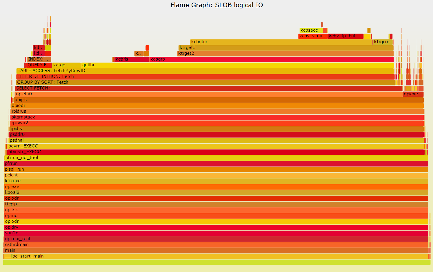
Similarly to what we discussed in the Example 1 above, we can now filter the stack traces to highlight the rowsource data. In addition in this example we also leave the details of the functions that start with the letter 'k', notably this includes the Oracle kernel function kcbgtcr (Kernel Cache Buffer Get Consistent Read).

Figure 5: Flame Graph of SLOB logical IO (8 concurrent sessions) where the stack data has been filtered to show only rowsource functions and functions stating with 'k'. See more details in the SVG version

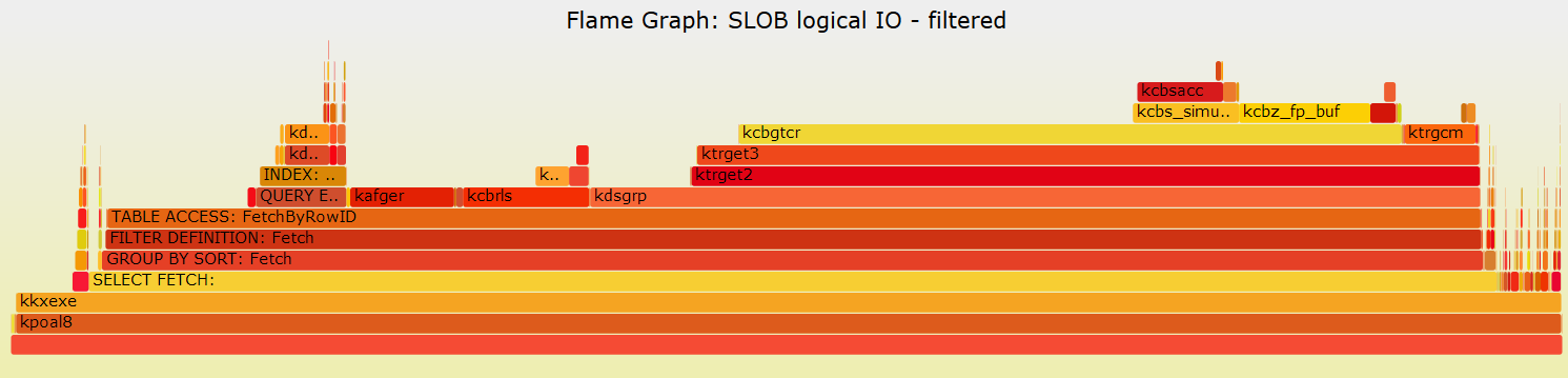
We can correlate the rowsource execution steps as we see them in in Figure 5 with the execution plan of the SLOB test query reported here below (Figure 6).

Figure 6: Execution plan of the SLOB query used for the tests described in this article.


How the Flame Graphs 4 and 5 have been generated

Test setup:

• See example 1 above on the details about downloading the FlameGraph scripts and about the requirements for perf and os_explain.sed
• Download SLOB and configure the test environment. 8 schemas have been used for the tests reported here. See also this post for additional details on testing with SLOB.
• Make sure that SLOB runs with all data in buffer cache. 8 schemas of 1M blocks each have been used for this tests and a buffer cache of 70 GB.
• To facilitate loading data into the buffer cache this SQL was run prior to testing:
• alter session set "_serial_direct_read"=never;
• alter table user1.cf1 cache;
• select count(*) from user1.cf1;
• repeat for the rest of the test users.
• while a SLOB test is running we can check that the workload is not doing physical IO for example using Tanel's snapper. For example: snapper all 10 1 "select inst_id, sid from gv$session where username like 'USER%'"

Test execution:

• Session 1: run the SLOB test. In the test case described here below I used 8 sessions (that is I started the test with ./runit.sh 8) 
• Session1: identify the PIDs of the server sessions running SLOB workload. For example use: select spid from v$process where addr in (select  paddr from v$session where username like 'USER%');
• Session 2: gather perf data for 20 seconds at default sampling rate (1 KHz):  perf record -g -a -p 51929,51930,51931,51932,51933,51934,51962,51963 sleep 20

Data processing and visualization:

• Generate the stack trace in a txt file: perf script >myperf_scriptSLOB.txt
• Create the flame graph: grep -v 'cycles:' myperf_scriptSLOB.txt|sed -f os_explain.sed|../FlameGraph-master/stackcollapse-perf.pl|../FlameGraph-master/flamegraph.pl --title "Flame Graph: SLOB physical IO" >Figure1_SLOB.svg
• Create the flame graph with only rowsource steps and k* function: grep -i -e qer -e opifch -e ' k' -e ^$ myperf_scriptSLOB.txt|sed -f os_explain.sed|../FlameGraph-master/stackcollapse-perf.pl|../FlameGraph-master/flamegraph.pl --title "Flame Graph: SLOB physical IO - filtered" >Figure2_SLOB.svg

Example 3: profiling multiple processes - physical IO

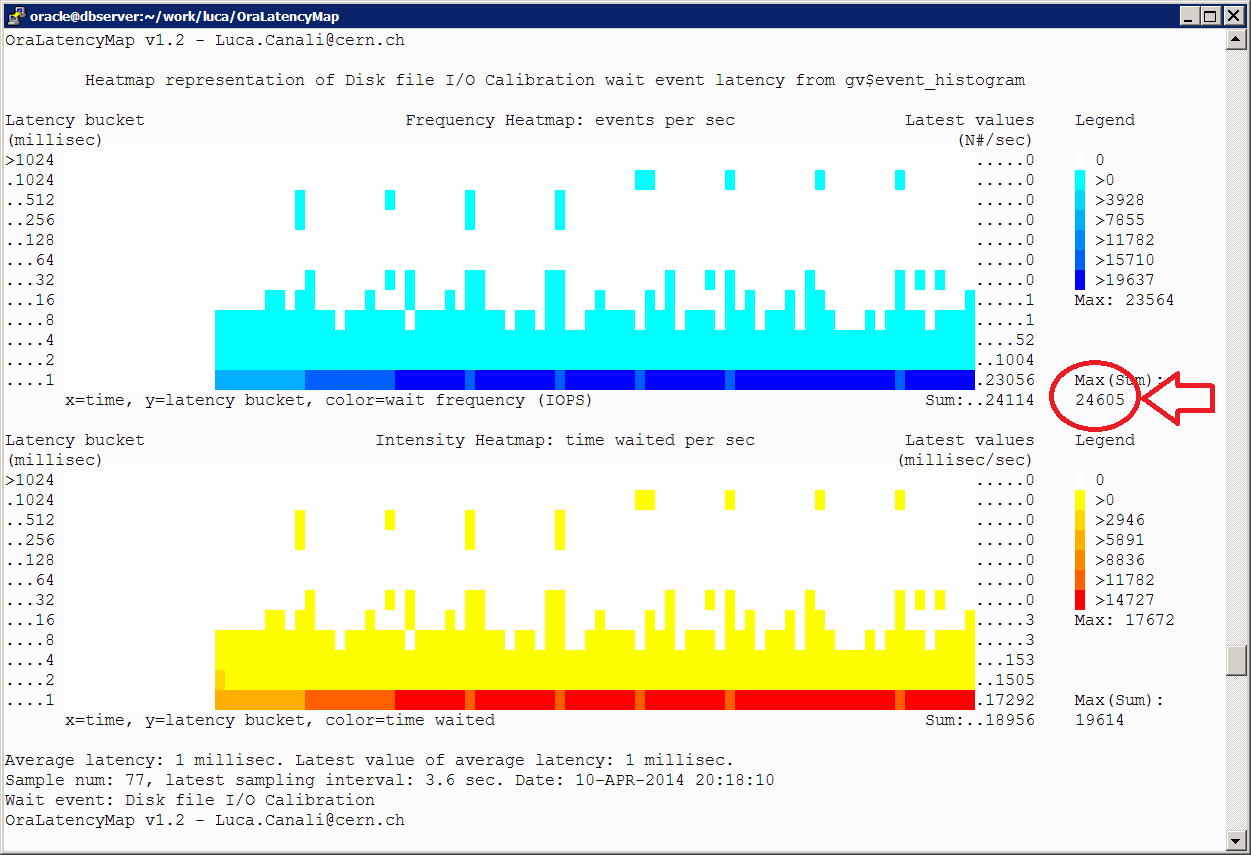
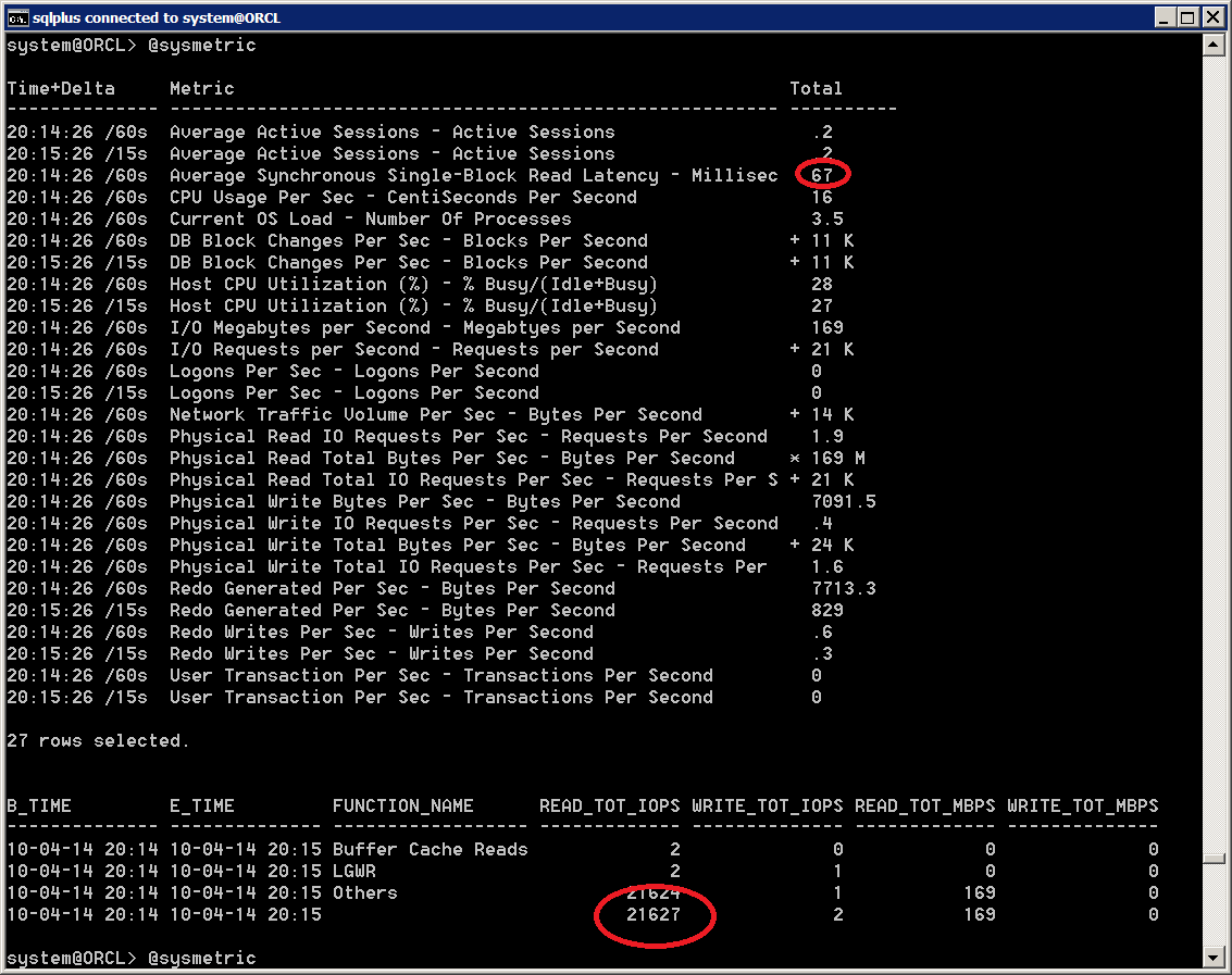
We will use the same SLOB workload as example 2 but this time with a very small buffer cache therefore forcing the DB to do physical I/O to read SLOB data from the storage. Random I/O reads will be instrumented by Oracle with the db file sequential read wait event (see also this post for additional details and examples on testing random I/O with SLOB).

Figure 7: Flame Graph of SLOB physical IO (8 concurrent sessions). See more details in the SVG version

By comparing Figure 7 (SLOB physical I/O) with Figure 4 (SLOB logical I/O) we notice that

• we have many more function calls in the case of physical I/O than in the corresponding graph with only logical I/O. Moreover in Figure 7 we can see several stack traces that contain only OS kernel calls and that cannot be easily associated with a particular step in Oracle execution. Note the system under tests used NAS storage so physical IO appears as network traffic.
• Moreover from the SVG graph versions we can count the number of samples stack traces and notice that in the case of physical IO we have considerably less values. This is because perf will only collect stack traces when the process is on-CPU.
• Another important fact that we notice is the appearing of Oracle kernel kcbzib function. This seems to be associated with reading blocks into the cache with physical reads.

Figure 8: Flame Graph of SLOB physical IO (8 concurrent sessions) where the stack data has been filtered to show only rowsources and functions stating with 'k'. See more details by hovering over the graph lines in the SVG version

Example 4: profiling the server workload

This example is about measuring and visualizing stack traces collected for on entire server. The interpretation becomes more complex as multiple workloads are measured together. Moreover system calls for I/O and other activities are measured as well.
Another important fact to take into consideration is the footprint of data collection. For this reason a reduced frequency of 99 HZ was used for sampling.

Data gathering at 99HZ for 20 seconds for the whole instance: perf record -g -a -F99 sleep 20

The steps for data visualization are the same as was used in Examples 2 and 3. Here below in Figure 9 the Flame Graph of the measured data and a 'filtered version' in Figure 10.

• Generate the stack trace in a txt file: perf script >perf_data.txt
• The commands used to generate the 'filtered' Figure 10 are: grep -i -e qer -e opifch -e ' k' -e exe -e ^$ perf_data.txt|sed -f os_explain.sed|../FlameGraph-master/stackcollapse-perf.pl|../FlameGraph-master/flamegraph.pl --title "Flame Graph - filtered" >perf_Figure10.svg

From the row source names reported in Figure 10 below we can guess what the workload on the server was, which types of operations were executed, with details on the queries, such as the access path used and on the type of DML. We can also measure which Oracle functions were executed for most of the CPU time. It's worth mentioning again that only on-CPU workload was captured.

Figure 9: Flame Graph of the workload of an entire server for 20 seconds, stack traces sampled at 99 Hz. See more details in the SVG version

Figure 10: Flame Graph of the workload of an entire server for 20 seconds, stack traces sampled at 99 Hz. where the stack data has been filtered to show only rowsources + functions stating with 'k' or containing 'exe' in their name. See more details in the SVG version

Conclusions

High-frequency sampling stack traces is a powerful technique to investigate process execution at the OS level, in particular for CPU-bound processes. This technique can be successfully applied to the study of Oracle performance and complex troubleshooting. It can complement and in some cases supplement the information exposed by Oracle's V$ views and wait event interface in general. Flame graphs are a visualization technique introduced by Brendan Gregg to facilitate the analysis of sampled stack data. The analysis of stack traces for Oracle processes currently relies on the little information available on the Oracle Support document "ORA-600 Lookup Error Categories" (formerly MOS note 175982.1, more recently seen with note 1321720.1) and on the published work of experts who have approached this field and published their findings, notably Tanel Poder. 
Much of the potential of these techniques is still untapped, we have covered in this article a few basic examples.

Additional resources on interpreting stack traces and on profiling Oracle rowsources and SQL execution can be found in Tanel's blog and Enkitec TV video and in Alexander Anokhin's blog.
More info on the use of Flame Graphs can be found in Brendan Gregg's blog.
See also on this blog a post about using Flame Graphs for investigating Oracle optimizer.

A Closer Look at CALIBRATE_IO

Topic: This blog entry is about investigating Oracle's DBMS_RESOURCE_MANAGER.CALIBRATE_IO

Spoiler alert: For quantitative analysis of storage performance and in particular for measuring random read I/O in Oracle, I'd rather advise the use tools that allow generating test workloads in a controlled manner, in a way that can be understood and measured and in particular with latency details together with IOPS measurements. For example SLOB by Kevin Closson is an excellent tool that I have happily used in several occasions for this purpose (see also this example). Kyle Hailey has also written on the topic of storage testing, see for example this. Brendan Gregg has written on the advantages of using the active benchmarking method.

What is DBMS_RESOURCE_MANAGER.CALIBRATE_IO? 
From the Oracle performance tuning manual: "The I/O calibration feature of Oracle Database enables you to assess the performance of the storage subsystem, and determine whether I/O performance problems are caused by the database or the storage subsystem."
This is promising and should definitely catch the DBA's attention. At a closer look it appears that CALIBRATE_IO can probably be better described as a simplified version of the Oracle ORION testing tool integrated inside the database with the goal of measuring key metrics of the database storage, namely the maximum throughput for read sequential IO and maximum IOPS for random read I/O. CALIBRATE_IO measures only read workload.

DBMS_RESOURCE_MANAGER.CALIBRATE_IO has a few advantages: it is very simple to use, it does not require any additional installation steps, it works in RAC and it produces a simple output.

CALIBRATE_IO attempts to measure random I/O performance with two numbers: maximum number of IOPS and average latency at which it is measured. Unfortunately this can be often misleading for many of the modern storage systems where the IOPS latency distribution is multi-modal, that is we have a fast speed for I/Os served by SSD (or RAM) cache and a slower speed for I/Os served by physical disks. 

Another shortcoming is that the workload generated by CALIBRATE_IO 'is a black box', we don't know the details of how the numbers that are reported in the output are measured and how the testing workload is generated. We will investigate CALIBRATE_IO workload in the rest of this article.

How to run CALIBRATE_IO, a sqlplus example:

Let's start with an example on how to run procedure (note the code below will generate high load on the storage for a few minutes, so you will probably want to be careful on where you run it).

SET SERVEROUTPUT ON
DECLARE
   lat  INTEGER;
   iops INTEGER;
   mbps INTEGER;
BEGIN
   DBMS_RESOURCE_MANAGER.CALIBRATE_IO (num_physical_disks=>100, max_latency=>100, max_iops=>iops, max_mbps=>mbps, actual_latency=>lat);
   DBMS_OUTPUT.PUT_LINE ('max_iops = ' || iops);
   DBMS_OUTPUT.PUT_LINE ('latency  = ' || lat);
   DBMS_OUTPUT.PUT_LINE ('max_mbps = ' || mbps);
end;
/

Input parameters:
The first input parameter num_physical_disks has been set to 100 in the example. From the documentation this parameter should be set to the "..approximate number of physical disks in the database storage. This parameter is used to determine the initial I/O load for the calibration run". Based on the observation of a few tests, I noticed that the procedure auto-calibrates the load so I confirm that it does not seem to be important to get this value right.
The second input parameter is max_latency: "Maximum tolerable latency in milliseconds for database-block-sized IO requests". For the tests described in this article I have typically used the value 100 (milliseconds). Lower values for this parameter may throttle the test workload as CALIBRATE_IO tries to meet this limit for the average I/O latency.

Output parameters:
The results of the measurements are three output parameters: max_iops, latency, max_mbps, as in the example above. The values are also made available in the view DBA_RSRC_IO_CALIBRATE (based on the underlying table SYS.RESOURCE_IO_CALIBRATE$). Notably an additional output parameter MAX_PMBPS "Maximum megabytes per second of large I/O requests that can be sustained by a single process" is only available in DBA_RSRC_IO_CALIBRATE.
MAX_IOPS and LATENCY output parameters are respectively "Maximum number of I/O requests per second that can be sustained. The I/O requests are randomly-distributed, database-block-sized reads." and "Average latency of database-block-sized I/O requests at MAX_IOPS rate, expressed in milliseconds".

Note: the results of the calibrate job can be deleted form the system with: delete SYS.RESOURCE_IO_CALIBRATE$ (and commit). See also this article by Gwen Shapira where also other oddities of CALIBRATE_IO and its relationship with the use of parallelism are discussed.

Investigations of CALIBRATE_IO workload

In the following we will go through the exercise of investigating  the workload from CALIBRATE_IO, taking it as a black box. It will be a simple but instructive way to get to practice some techniques for investigating I/O in Oracle and to further understand what CALIBRATE_IO can do for us and what are its limitations. 

- Start calibrate I/O and observe the processes that are executing the workload.
For investigating this I will use a script that queries from V$SESSION or V$ACTIVE_SESSION_HISTORY. For example top.sql and ash.sql that I have described in the article at this link.

The result is that CALIBRATE_IO spawns a certain number of slaves called CS00, CS01,... The CSXX slaves will be spawned on each active Oracle RAC instance. The number of CALIBRATE_IO processes spawned per instance is equal to the value of the parameter CPU_COUNT, at least in the few tests I have run on a few servers with different numbers of CPUs and consequently of CPU_COUNT, ranging from 8 to 32. The number of slaves that are active at a given time however fluctuates over time as the test progresses. Another fact that we can immediately see is that there is a special wait event triggered by CALIBRATE_IO slaves when doing I/O: "Disk file I/O Calibration"
Here below an example taken from a 4-node RAC database:

- What type of I/O is issued by CALIBRATE_IO?
We can investigate this for example by querying GV$IOFUNCMETRIC with a script such as iometric_details.sql that I have also mentioned in the post at this link.

The results is that CALIBRATE_IO first generates random I/O for small block reads on all RAC nodes, then sequential large I/O reads from multiple sessions and nodes, finally sequential large reads using a single session. This behavior is consistent with the documentation and the tool's output.
Here below an example of monitoring CALIBRATE_IO run on a 4-node RAC during the first execution phase (small random I/O reads). We can see that all nodes are performing I/O for small random read and that the grand total of IOPS is about 30K.

Another example here below is from the same 4-node RAC during the second execution phase, we can see that all four nodes are now executing large sequential reads for a grand total of about 2.5 MB/sec.

- How is the I/O distributed across the storage?
The workload from CALIBRATE_IO is a black box, however we can imagine that the tool uses the existing data files for generating the load. We want to confirm that with some direct investigations: we can query GV$IOSTAT_FILE to get the number of single block requests at the start and at the end of the test workload. By calculating the differences we can see which files have been read. The result is that CALIBRATE_IO reads from all the files in the database. Approximately the amount of blocks read that I have measured is proportional to the file size, that is CALIBRATE_IO spreads the load uniformly across the DB files and filesystems used.
An important fact to keep in mind is that if we use more filesystems/storage types for our database files, CALIBRATE_IO will measure all of them at the same time and produce a result that is an average value.
An example of the type of query that we can use to see which files are being read is:

- CALIBRATE_IO is expected to use asynchronous I/O, can we confirm it?

Using Linux strace on a database using ASM storage over block devices, we can see that I/O is performed using the async IO system calls: io_submit and io_getevents. For the random I/O workload reads are of 8KB, for the sequential I/O workload, reads are of 1MB. This was expected. 

However we can also see that each CSXX slave of CALIBRATE_IO submits I/Os one by one and then most of the time an io_getevents follows immediately reaping 1 I/O. There are exceptions where larger numbers of I/O are reaped together (for example 128 8K I/Os), this latter case shows the true nature of asynchronous I/O for CALIBRATE_IO.

In the second and third part of the workload, CALIBRATE_IO tests for large sequential reads, in this case we see io_submit calls with a payload of 1MB, as expected.

Given the asynchronous nature of the I/O, the latency details for the wait event "Disk file I/O Calibration" do not always give us a precise indication of the I/O service times. In some cases CALIBRATE_IO slaves will issue an I/O and wait till it has been ripped, providing us the service time information as a wait event duration. For high-load tests CALIBRATE_IO may issue many IO requests (typically one by one) but reap them in bunches, as mentioned also in the paragraph above. There the wait event duration becomes uncorrelated with I/O service time. We can see here below an heat map of the waits, where most of the waits appear in the 1ms bucket. This is an artifact of the way Oracle times this wait event (if you are interested in Oracle timing of asynch I/O events, see the excellent investigations by Frits Hoogland in his blog).

These are some key metrics taken during the execution of CALIBRATE_IO for this system with 204 SATA disks, RAC, but running on a single node for this test:

- Can we trust the results from CALIBRATE_IO?

As a reference the result of the CALIBRATE_IO run on the system discussed above with 204 SATA disks in JBOD configuration (Oracle 11.2.0.3 on Linux) was:

max_iops = 24211

latency  = 5

max_mbps = 780

The max IOPS number and max MBPS are the expected values. This was a JBOD without any relevant amount of RAM nor SSD cache. The expected value for max IOPS is basically just another way of counting the number of disks (something north of 100 IOPS per disk on this hardware). Also the expected value for sequential I/O is easy to estimate in about 800MB/s (FC HBA, 2 ports at 4Gig each). Therefore the values for max IOPS and max MBPS measured by CALIBRATE_IO for this system agree with expectations.

However, the measured latency value appears to be too small and probably an artifact of using async I/O.

Here below we can see a test performed, on the same system, with SLOB where we get a better drill down of latency and understand what is happening (high latency exposed, effects of saturation due to high load and to aging disks resulting in I/O outliers, etc). IOPS measurements without latency details do not give us the full picture!

In the figure here below we can see some key metrics taken during the execution of SLOB. In particular note the number of IOPS (21K), which is similar to the previous max IOPS value measured with CALIBRATE_IO. However the average Synchronous IO latency (35 ms on that particular snapshot), is much higher than what reported by CALIBRATE_IO. More details of the measured synch IO latency can be seen in the heatmap above.

- Comments on comparing the two tests for the JBOD case: 

The maximum number of IOPS measured when running SLOB turns out to be about the same as what is reported by CALIBRATE_IO for this particular system. This can be explained as the storage system under study is a JBOD and does not have multi-modal response time (there is very little RAM cache and no SSD cache on the storage system, so almost all I/O are served by spindles).

There is an important difference between the results of the two tests and it is with the latency details. Latency tells us many details about how the IO is being served by our storage. By measuring the latency using V$EVENT_HISTOGRAM and plotting is as a heatmap we can see that the system under study suffers from very high latency. It was indeed a very old system with aging disks (being decommissioned, BTW). We did not get the latency details from the CALIBRATE_IO run, which actually told us the average latency was 5ms at 21K IOPS! That would be quite a good result, however it is not the case in the reality and CALIBRATE_IO cannot be trusted on the latency measurement.

- More comments on CALIBRATE_IO and results for other systems types

I have run a few more measurements of CALIBRATE_IO on a NAS system equipped with SSD cache. I have compared the results of CALIBRATE_IO on those systems with values measured when running SLOB, with estimates based on the HW specs, and with estimates based on measurements on similar systems. The results have quite mixed: in some cases CALIBRATE_IO would report a value of max IOPS that was in the range of the expected values, in some other cases it would report a higher values (up to a factor 3 higher).
Latency values have proven once more to be quite important and possibly a key to understand what is happening: in the cases where max IOPS values were above the expected value, the reported latency was very low, the measured latency was reported to be 0 in some cases!
What is likely to happen is that the SSD cache of the controller is being exercised and CALIBRATE_IO does not realize that.

In conclusion for the tests run on NAS storage with SSD cache, CALIBRATE_IO cannot be trusted on the measurement of IOPS and latency.

Also the measurement of the maximum throughput for sequential I/O on this systems have been consistently below the expected value. We expect 1 GB/sec of maximum sequential I/O throughput for this HW, this is confirmed by some simple tests with parallel query, however in most cases CALIBRATE_IO would report only about 500 MB/sec and therefore for this system it cannot be trusted on the measurement of sequential I/O throughput.

Conclusions:

In this post we have investigated the use of CALIBRATE_IO to produce I/O intensive workloads for testing storage for Oracle read workloads. CALIBRATE_IO is an easy tool to use and allows to get started with testing very quickly. However CALIBRATE_IO fails to produce accurate results in many circumstances. In particular some important shortcomings of CALIBRATE_IO are: the workload is a black box, we cannot easily scale up the load and understand the effects of storage RAM or SSD cache in the results, it does not provide a latency breakdown of the I/O, therefore hiding some critical details on the storage behavior. Moreover the results of the measured max IOPS, max MBPS and the provided latency values are not always accurate. Finally, by design CALIBRATE_IO will only measure a single value of max IOPS and this can be misleading for storage system with multi-modal response times (such as storage based on disks for capacity but with large amounts of SSD cache).

See also additional links to tools and methods for storage performance studies provided in the first part of the article.

Recent Updates of OraLatencyMap and PyLatencyMap

Topic: This post introduces the latest changes to OraLatencyMap and PyLatencyMap, two custom tools for collecting and displaying Oracle wait event latency details using heatmaps.

OraLatencyMap is a SQL*Plus tool, with a core written in PL/SQL, aimed at studying Oracle random I/O by displaying the latency drill-down of the wait event 'db file sequential read' using heatmaps. The tool can also be used to collect and display event latency histograms for any other Oracle wait event, for example: log file sync to study commit time latency.

Additional info: Hotsos conferenece 2014 presentation "A Latency Picture is Worth a Thousand Storage Metrics".

OraLatencyMap v1.2 (March 2014) introduces the following improvements:

• A legend for the color palettes is displayed on the right side of the heatmaps
• Average latency values are displayed in the graph footer: a global average (across all data in the plot) and the latest value of the average are calculated from v$event_histogram and displayed.
• More example scripts are packaged together with the tool, including a script for the analysis of 'log file sync' wait event latency and a script for Exadata storage for the latency drill-down of the wait event 'cell single block physical read'.

An example of the output of OraLatencyMap v1.2 can be seen in the screenshot here below:

Download: OraLatencyMap can be downloaded from https://github.com/LucaCanali/OraLatencyMap

---

PyLatencyMap v1.1 (March 2014) introduces the following improvements:

• Average latency values are displayed in the graph footer: a global average (across all data in the plot) and the latest value of the average are calculated from v$event_histogram and displayed.
• More example scripts are packaged, including a script for Exadata storage for the latency drill-down of the wait event 'cell single block physical read'.

PylatencyMap is the Python version of OraLatencyMap. It provides additional features, mostly related to the integration with multiple input data sources: 10046 trace files, AWR data,  DTrace data, replay of measured data.

Download: PyLatencyMap can be downloaded from https://github.com/LucaCanali/PyLatencyMap 

Wait Event History Sampling, an Experiment in Oracle Performance Analysis

Topic: This post is about a performance analysis technique based on high frequency sampling of wait event history data in Oracle. Two scripts are provided for performing this type of analysis and two example cases are discussed applied to the study random read latency and read workload characterization.

Context: In the context of performance analysis, for example for a study of I/O response time, I want to analyze the flow of all wait events for 'db file sequential read', say for a group of sessions. What are the options?

• 10046 trace is the classic way. This provides all the details of the SQL execution including wait event details if I want to. One of the problem here is with the scalability of writing into trace files especially if I want to trace many and very active sessions, in addition possibly tracing for a long time. Moreover the amount of data in the traces is an overkill for what I need, as I am interested only in some particular aggregations of db file sequential read wait events.
• DTrace of Oracle sessions provides an elegant and direct way to tap into the wait event interface for real-time analysis (see this article for details). However this method is still niche and works best in Solaris, while I mostly work with Oracle on Linux.
• Sampling is a typical alternative to tracing. Oracle ASH does just that and is a great source of performance data. However Oracle ASH data is sampled at 1 Hz, too slow for capturing I/O events. (Note: ASH sampling rate can be increased by tweaking _ash_sampling_interval, although the highest available rate currently is 10 Hz, still too low for our purposes).

Sampling of wait event history data

Oracle's V$SESSION_WAIT_HISTORY provides details of the last 10 wait events for each session currently connected to the instance. The idea is to use this data as a series of ring buffers, indexed by Oracle's SIDs. How can we wrap around the buffers? It turns out that the underlying X$KSLWH table has a column that can be used just for that: KSLWHWAITID (the values in KSLWHWAITID are not reported in V$SESSION_WAIT_HISTORY unfortunately). Here below an example of some of the columns of interest in X$KSLWH:

KSLWHSID	KSLWHWAITID	KSLWHETEXT	KSLWHETIME	KSLWHP1	KSLWHP2	KSLWHP3
42	21016	db file sequential read	300	25	148935	1
42	21015	db file sequential read	1020	25	47683	1
42	21014	db file sequential read	16024	25	124765	1
42	21013	db file sequential read	4100	25	57668	1

Example 1: fine-grained wait event latency histograms 

Let's put our sampling technique at work for capturing latency data and then display the collected data with latency histograms. Note: latency histograms and their graphical representations are useful for studies of random read performance, see also this previous article on the subject.

The advantage of the method based on sampling X$KSLWH over the use of  V$EVENT_HISTOGRAM are:

• The lowest bucket in V$EVENT_HISTOGRAM is 1 ms, which is too coarse for I/O coming from SSDs. By sampling we can reach to a finer scale (depending on the sampling rate, in practice ~100 micro seconds is easily reachable).
• We can apply a finer grain selection to the sessions we want to investigate, for example by limiting our sampling to one session or a group of sessions, as opposed to measuring the entire instance.

The tool: event_history_sampler_histogram.py is a python script that I wrote for this type of analysis. The script works by sampling X$KSLWH in a tight loop (which also mean it is CPU hungry). Here is a screenshot of the usage of this script with its options:

Here an example of the tool in actions with its output:

This script can be easily interfaced with PylatencyMap for heat map visualization. Here below is an example applied to displaying latency data of a workload generated with SLOB (note that the latency measurements are in microseconds):

$ python event_sampler_latency_histogram.py --sql="username like 'USER%'"|python ../PyLatencyMap/LatencyMap.py

Example 2: real-time analysis of all I/O instrumented by db file sequential read 

The use case here is to analyze all the I/O performed via db file sequential read and perform real-time analysis of the data. This is similar to the case above but instead of limiting the analysis to the latency time we want also to make use of the information on which blocks have been read.
For example we can record all the blocks that have been read and instrumented using db file sequential read in addition to their latency details. Details of the block read are available as wait event parameters p1 and p2 (file number and block number respectively). We can collect the data using a technique similar to what was described above for the latency histograms example: that is by sampling X$KSLWH.

Some examples of what can we learn from this type analysis:

• We can collect the list of all the blocks read in a given time interval. One of the simplest analysis is to count how may distinct blocks we have read. This gives an indication of how big the active area of the data set is for this workload. 
• We can use the information on the size of the active data set as help for sizing the cache (for example for sizing the needs for SSD cache in the storage, or sizing the amount of RAM needed for efficiently buffer the workload).
• We can study physical IO based on latency, for example by measuring how much of the workload is reading 'new blocks' or instead reading multiple times the same set of data blocks.
• In the example below you can see that for each sampling interval (the default is a 10-second interval) we have info on:
• the number of distinct blocks sampled since the script has started collecting 
• the number of blocks read during the latest collection interval having a latency <2 ms (presumably from SSD cache) and the drill-down details of whether they are new block reads or blocks that have been read before during sampling
• same as above but for blocks read with latency >=2 ms (presumably I/O coming from spindles) 
• It's also straightforward to add custom analysis code in the python script to provide for different use case, if needs arise.

Here below an example screenshot of test analysis performed with a python script I wrote called event_sampler_gather_IO_history.py:

$ python event_sampler_gather_IO_history.py --sql="username='MY_APP_USER'"

Limitations and additional comments

The main limitation of this method lies in the necessity to sample at high frequency, the higher the frequency the more events with low latency we can capture. In practice a frequency of 1 KHz seems good enough for the study of random reads. However this also means running the script in a 'tight loop' and consuming 1 core of CPU constantly during the execution of the script.
Moreover the execution time of the sampling query depends on the number of sessions monitored, therefore we will see lowering sampling rates as we increase the number of sampled sessions. In practice sampling up to a few hundred concurrent sessions at a time seems to give still good results.
Another limitation is due to the fact that we are only sampling db file sequential read waits and ignoring other wait events such as db file parallel read or in general multi-block and/or async IO events.
The script event_sampler_gather_IO_history.py works by collecting information on all blocks read during its execution. In the example above where information of 12M blocks was stored in a python dictionary, almost 2GB of RAM were used. The memory footprint of the script should be optimized in a future version, in the mean time memory consumption needs to be monitored when running this type of analysis.
Note for RAC: these scripts will only monitor activity in the instance where they are connecting to (basically it's like using V$ views as opposed to GV$).

Download the scripts:

The scripts mentioned in this blog are available from http://cern.ch/canali/resources.htm

Feel free to download and try them out, however beware that they are still in a beta stage.

The scripts have been tested against Oracle 11.2.0.3, 11.2.04 and 12.1.0.1 on Linux RHEL5 and RHEL6 with Python 2.4 and 2.6 and cx_Oracle version 5.1.2.

Conclusions

This article describes the main ideas of a technique for performance analysis of Oracle wait event data based on sampling the wait event history data and in particular X$KSLWH to produce a wait event data stream for real-time analysis. This has been illustrated with two examples related to to the study of random read latency and to the study of random IO patterns. The scripts used for this analysis are written in python and available for free download.

Clusterware 12c and Restricted Service Registration for RAC

Topic: This post is about exploring the mechanisms used by Oracle Clusterware 12.1.0.1 to restrict remote service registration, i.e. the 12c new feature "Restricting Service Registration for Oracle RAC Deployments"

Why is this useful? This improvement of 12c clusterware and listeners over the 11.2 version is useful mainly for security purposes, for example as a measure against TNS poisoning attacks (see also CVE-2012-1675), and it is particularly relevant for RAC deployments. Another important point is that it makes the DBA job easier by avoiding the complexity of COST (Class of Secure Transport) configurations (see also support Doc ID 1453883.1).
Notably Oracle 11.2 databases can profit of this 12c improvement too (in the case where the 11g RAC database installed under 12c clusterware).

Spoiler: If you have heard already about the 12c new feature of valid node checking for registration (VNCR) you are still in for a surprise.

Listeners in Oracle RAC in 11.2 and 12.1:
There have been important changes on how listeners are used in RAC starting with the clusterware 11.2. The details are discussed in a previous post. The main points are that (1) we now have local listeners and scan listeners, all using the same binary tnslsnr but with different scope. (2) Most of the listener configuration parameters, in RAC, are taken care of by the clusterware (Oraagent).
Database instances will perform remote service registration to remote listeners as specified by the instance parameter remote_listener (BTW remote service registration is needed to enable the server-side load balancing mechanism of RAC). PMON takes care of the registration in versions up to 11.2, in 12c a new LREG process has been introduced. Local service registration is configured at the instance level using the parmeter local_listener. Normally we will leave its value unset and the clusterware (Oraagent) will take care of setting it to the address of the local listener.  In 11.2 and higher the parameter listener_networks is also relevant, typically in the case of setups with more than one public network (the details are outside the scope of this discussion).

Why restricting service registration?
If service registration is not restricted, anybody who can reach the listener via the network can register a service with it. This opens the way to abuses, such as crafting an attack aimed at redirecting legitimate TNS traffic towards the attacker's machine (see also TNS poisoning attack mentioned above).

What's new in 12.1.0.1?
After performing a 12.1.0.1 vanilla RAC installation we notice that the scan listeners will only accept remote registration over TCP from local cluster nodes. This is an improvement over 11g where to obtain the same result the DBA had to manually execute a series of steps for COST (Class of Secure Transport) configuration, in order to configre the TCPS protocol to restrict remote registration. This improvement is listed as a new feature of 12c for RAC as "Restricting Service Registration for Oracle RAC Deployments".

How does 12c restrict service registration?
In $GRID_HOME/network/admin we can examine listener.ora: we notice a few additional lines from the equivalent file in version 11.2 (see also this post for more details on listener.ora in 11.2), that is lines containing valid node checking configuration. For example:

VALID_NODE_CHECKING_REGISTRATION_LISTENER=SUBNET # line added by Agent
VALID_NODE_CHECKING_REGISTRATION_LISTENER_SCAN1=OFF # line added by Agent

VALID_NODE_CHECKING_REGISTRATION_LISTENER_SCAN2=OFF # line added by Agent

With the first of those lines listed here above the clusterware (OraAgent), which takes care of most of the listener configurations, informs us that after starting the listener it has also connected to it (via IPC) and activated the new feature of valid node checking for registration (VNCR) for the listener called LISTENER, that is for the local listener.
What VNCR does is to restrict remote service registration, in this case to the local subnets.  A short recap for the possible values for the VNCR from support Note Id 1592571.1 is listed here below. See documentation for further details.

• OFF/0 - Disable VNCR
• ON/1/LOCAL - The default. Enable VNCR. All local machine IPs can register.
• SUBNET/2 - All machines in the subnet are allowed registration. This is for RAC installations.

What about the scan listener?
From the snippet of listener.ora reported above we can also see that VNCR is surprisingly turned OFF for the scan listeners (at least in this configuration that I have obtained after a vanilla 12.1.0.1 clusterware installation). However, as we can easily check (see more on techniques below) remote service registration to the scan listeners is indeed restricted and not possible for servers outside the RAC cluster. Therefore another mechanism, different from VNCR, is in place for scan listeners. Let's investigate!

Some explanations:
It turns out that the clusterware (OraAgent) does again the work, but this time without making it visible with an entry it in listener.ora. OraAgent takes care of setting the parameter REMOTE_REGISTRATION_ADDRESS for the scan listener, setting a endpoint for it on the HAIP network. Note, for more info on HAIP see documentation and support Doc Id 1210883.1
A log of this listener parameter change can be found in the logfile of the Clusterware Agent (OraAgent for crsd): $GRID_HOME/{NODE_NAME}/agent/crsd/oraagent_oracle/oraagent_oracle.log). The result can also be observed by using lsnrctl:

$ lsnrctl show remote_registration_address dbserver1-s:1521

Connecting to (DESCRIPTION=(CONNECT_DATA=(SERVICE_NAME=))(ADDRESS=(PROTOCOL=TCP)(HOST=xx.xx.xx.xx)(PORT=1521)))
dbserver1-s:1521 parameter "remote_registration_address" set to (DESCRIPTION=(ASYNC_TIMER=yes)(EXPIRE_TIME=1)(TRANSPORT_CONNECT_TIMEOUT=15)(ADDRESS_LISTDRESS=(PROTOCOL=tcp)(HOST=169.254.163.245)(PORT=11055))))

What does REMOTE_REGISTRATION_ADDRESS do?
When the listener receives a remote registration request it will reply to the client (which would normally be Oracle's PMON or LREG process) with a request to re-send the registration message via the HAIP network, in the example above: (HOST=169.254.163.245)(PORT=11055). This would only be possible if the instance trying to register its services has access to the same cluster interconnect (that is if it belongs to the same RAC cluster or to another RAC cluster which shares the same private network).
The default value for REMOTE_REGISTRATION_ADDRESS is OFF, therefore the redirection mechanism described here above is not in place unless explicitly activated (by the 12c clusterware in this case). See also this link at the documentation for REMOTE_REGISTRATION_ADDRESS.

VNCR can be used for scan listeners too. 
VNCR appears to be used when an invited list is specified. That is for the case when we want to further restrict the nodes allowed to perform remote service registration. An example here below of how this can be done, see the documentation for details:
$ srvctl modify scan_listener -update -invitednodes dbserver1,dbserver2

After doing this change we will notice that (1) VNCR (valid node checking) is now used for the scan listeners. (2) That the invited nodes are limited to the listed nodes and local subnet. (3) That the parameter remote_registration_address is no longer used in this case. Here below a relevant snippet from listener.ora:

VALID_NODE_CHECKING_REGISTRATION_LISTENER_SCAN1=SUBNET  # line added by Agent

REGISTRATION_INVITED_NODES_LISTENER_SCAN1=(dbserver1,dbserver2) # line added by Agent

Additional comments on configuring VNCR for RAC 

With the clusterware version used for these tests (12.1.0.1) I was not able to set VALID_NOTE_CHECKING_REGISTRATION_LISTENER to the value ON using srvctl, but rather Oracle was using the value SUBNET. The value ON is a more restrictive value than SUBNET (see  discussion above) and I believe it is more appropriate for most cases as a setting for the local listener.
In a test system I have noticed that when manually editing VALID_NODE_CHECKING_REGISTRATION_LISTENER=ON in listener.ora, the change would stay persistent after listener restart.
Moreover in 12.1.0.1 clusterware, when specifying a list of invited nodes for the scan listener (as in the example above), the VNCR parameter will be set to SUBNET rather than to ON. In this case a manual update of VALID_NODE_CHECKING_REGISTRATION_LISTENER_SCAN1=ON did not prove to be persistent after scan listener restart (OraAgent would overwrite the value).

Some pointers to investigation techniques

How to test if a listener will accept remote service registration:
We can use a test database as the 'attacker' and set the remote_listener parameter to point the listener under test. This will send a remote service registration request from the 'attacker' instance (from PMON or LREG depending on the version) towards the target listener. This operation and its result will be visible in the target listener's listener.log file. If the registration has been successful it will also be visible by running the command lsnrctl services target-listener:port.
A basic example showing how to set the remote_listener parameter:
SQL> alter system set remote_listener = '<endpoint>:<port>' scope=memory sid='*';

Listener configuration details from the clusteware logs:

Most of the parameters for the listener in 11.2 and 12c clusterware are set by the clusterware (for those parameters the configuration in the clusterware takes precedence from the values set in listener.ora). The log file of interest to see what operations have been performed by the clusterware to the listeners is the crsd oraagent log file: $GRID_HOME/{NODE_NAME}/agent/crsd/oraagent_oracle/oraagent_oracle.log

Listener logs tailing
The listener log files are an obvious source where we can get information on what is happening with remote registration.
Here below an example of listener.log entries generated following a remote registration request blocked by VNCR:
Listener(VNCR option 2) rejected Registration request from destination xx.xx.xx.xx
DD-MON-YYYY HH:MI:SS * service_register_NSGR * 1182
TNS-01182: Listener rejected registration of service ""

Network connections
When the clusterware sets remote_registration_address to provide redirection of the remote registrations, it will also set up an additional endpoint for the scan listener in the HAIP network. Moreover LREG (or PMON in 11.2) of remote instance can be seen to connect to this endpoint. Netstat is a handy tool to expose this. Example:
$ netstat -anp|grep tcp|grep 169.254

tcp   169.254.143.245:57688  0.0.0.0:*             LISTEN      12904/tnslsnr
tcp   169.254.143.245:57688  169.254.80.219:23239  ESTABLISHED 12904/tnslsnr

Trace Oracle processes
A simple technique to see the messaging between pmon/lreg while registering to the remote listener is to use strace. For example we can identify the pid of PMON (or LREG as relevant) and run: strace -s 10000 -p <pid>  (see above the syntax for alter system set remote_listener to trigger remote registration). Example from the output:

read(23, "\0\315\0\0\5\0\0\0\0\303(DESCRIPTION=(ASYNC_TIMER=yes)(EXPIRE_TIME=1)(TRANSPORT_CONNECT_TIMEOUT=15)(ADDRESS_LIST=(ADDRESS=(PROTOCOL=tcp)(HOST=169.254.163.245)(PORT=19771)))(CONNECT_DATA=(COMMAND=service_register_NSGR)))", 8208) = 205

Listener tracing
Another usefult technique is to set the tracing level for the scan listener to level 16 and look at the trace file, for example while triggering service registration. Example of how to set the trace level:

$ lsnrctl 
LSNRCTL> set current_listener dbserver1-s:1521
LSNRCTL> set trc_level 16

Conclusions
Oracle Cluserware 12c new feature "Restricting Service Registration for Oracle RAC Deployments" allows to restrict service registration for security purposes and to reduce the complexity of RAC installations. This new feature can be utilized by 12c and 11g RDBMS engines installed under 12c clusterware. This article investigates the details of the implementation of restricted service registration. One of the finding is that Oracle Clusterware does most of the configuration work in the background by setting the relevant parameters for the local and scan listeners.
A new 12c listener.ora parameter, REMOTE_REGISTRATION_ADDRESS, is used to secure scan listeners, at least in the case of a 12.1.0.1 vanilla clusterware installation. Another mechanism to restrict service registration is used for local listeners and for scan listener in particular cases: Valid Node Checking for Registration (VNCR), also a new feature of 12c.

How to Recover Files from a Dropped ASM Disk Group

Topic: This post describes a few tips and techniques on how to recover ASM files from a dropped disk group and an example of how to 'undrop' an ASM disk group

Context: This research stems from a recent case I have investigated where the data disk group of a test DB had all the disks with header_status 'FORMER': in other words the disk group had been dropped and hence could not be mounted. The next logical steps would have been to recreate the disk group and the test DB contained therein, although I first wanted to see if my 'favorite ASM support tools' (kfed and admu, see also references) could be of help to recover the lost files. It turns out that it is quite easy to recover files in a dropped diskgroup as the drop operation seems to just flick a key value in the disk headers. But let's go by steps:

Read files from a dropped ASM diskgroup with amdu

amdu is a diagnostic utility shipped with Oracle installations since 11g (can also be used for 10g, see references). It allows to read data from unmounted diskgroup and can be used in various support-type operations. For the case in question we can read files from a dropped diskgroup with

$ amdu -dis '/dev/mapper/MYLUN*p1' -former -extract ORCL_DATADG.256

This command will extract ASM file number 256 from the unmounted diskgroup ORCL_DATADG physically accessible from the path /dev/mapper/MYLUN*p1 (edit the LUN path as relevant for your system). File 256 in the ORCL_DATADG diskgroup in this example is the control file of the test database we want to recover.
Note: ASM starts numbering user-visible files from 256 (lower file numbers are used for the ASM system files, often hidden, see also X$KFFIL and more details in the references). It is very likely that file number 256 is a controlfile in 10g and 11g systems, as the controlfile is often the first file created in a disk group used for Oracle DBs. I have just observed a brand new 12c databases that file number 256 is the password file (new 12c feature), in that system the DB controfile is file number 257. 
The outcome of the amdu command above is to extract a copy of the file into the local file system (in a custom created directory). From the controlfile we can easily get a list of the rest of the DB files if needed. For example we can used the command string on the restored controlfile and process the output to find the name of the rest of the DB files.

Where are we with our disk group recovery? We have demonstrated a simple method to extract any file from a dropped disk group. Good news, we could recover the entire 'lost DB' onto a local filesystem.
Can we do better than that, for example recover all the files in one go and into ASM?

Undrop an ASM diskgroup with kfed

kfed is another great ASM diagnostic and repair tool shipped with Oracle. It allows to read and write ASM metadata from the disk header structures. Obviously writing into ASM disk headers is an unsupported activity that we can do at our own risk (or rather under guidance of Oracle support if needed).
Block number 0 of ASM allocation unit number 0 (see references for details) of each ASM disk contains, among others, a key called kfdhdb.hdrsts. Dropped disks have kfdhdb.hdrsts=4 (KFDHDR_FORMER), while disks that are members of a diskgroup have kfdhdb.hdrsts=3 (KFDHDR_MEMBER).
The 'trick' here is to read all the disk headers, one by one with kfed, change the value of kfdhdb.hdrsts from 4 to 3 and write the headers back into the disks.
Let's see this with a simple example, where we first create a diskgroup and then we dropp it to test the undrop procedure. The following assumes using a mixture of sqlplus commands on ASM and DB instances and running kfed from the OS prompt, as indicated.

1. Test setup

We create an ASM  disk group for testing, add a DB tablespace to it and then drop the diskgroup to prepare for the next step (undrop see point 2 below).

ASM_INSTANCE> create diskgroup ORCL_TESTDG external redundancy disk '/dev/mapper/MYLUN1_p1';

ORCL_DB> create tablespace testdrop datafile '+ORCL_TESTDG' size 100m ;

ORCL_DB> alter tablespace testdrop offline; -- this is needed or else diskgroup drop will fail as you cannot drop a diskgroup with open files

ASM_INSTANCE> drop diskgroup RDTEST2_TESTDROP  including contents;

2. Example of how to undrop the disk group and recuperate its files

We read the block header for each disk of the diskgroup (1 disk only in this example) and copy it to a local file:

$ kfed read /dev/mapper/MYLUN1_p1 aunum=0 blknum=0 text=dumpfile_MYLUN1_p1

Manual edit of the local copy of the header block:

$ vi dumpfile_MYLUN1_p1

replace the line:
kfdhdb.hdrsts:                        4 ; 0x027: KFDHDR_FORMER

with:
kfdhdb.hdrsts:                        3 ; 0x027: KFDHDR_MEMBER

We write the modified block header for each disk of the diskgroup (1 disk only in this example):

$ kfed write /dev/mapper/MYLUN1_p1 aunum=0 blknum=0 text=dumpfile_MYLUN1_p1


3. We can now check that our disk group and its files are back:

ASM_INSTANCE> alter diskgroup RDTEST2_TESTDROP mount;
ORCL_DB> alter tablespace testdrop online; 

Note, this procedure has been tested on Oracle for Linux, versions 11.2.0.3 and 12.1.0.1.

References

ASM internals and diagnostic utilities are a fascinating topic of investigation. An extensive source of information is the blog: ASM support Guy.
Some older research material that I have published on this topic can be found at wiki page on amdu and kfed and at wiki page on investigations of ASM internals.

Conclusions

We have discussed a few tips on how to read and recover files from a dropped disk group using the amdu utility and went through the main steps of an example procedure showing how to 'undrop' an ASM disk group using kfed.

UKOUG Tech13, Latency Investigations and Lost Writes

I am looking forward to participating again to the UKOUG annual conference. This year I will present together with my colleague Marcin Blaszczyk on two topics that are follow-up of articles in this blog.
The first talk is: Storage Latency for Oracle DBAs. A presentation about a performance tuning techniques for Oracle and storage, based on the study of latency wait event histograms and their representations with heat maps. It will be a good occasion also to show examples of the usage of OraLatencyMap and PyLatencyMap.
The second talk is: Lost Writes, a DBA’s Nightmare? This is a short presentation about lost writes in Oracle, based on our production experience. It's still surprising to me how such a seemingly unimportant failure class can in reality generate very complex failure and recovery scenarios.
If you are participating to the Tech13 conference, feel free to come and talk to us! Our presentations are on Monday morning (11:30 in the hall Exchange 4/5) and Wednesday morning (9:30 in the Exchange Auditorium).
More presentations at Tech13 by CERN colleagues: "Next Generation GoldenGate vs. Streams for Physics Data", "Cardinality Feedback Tuning Revisited – Adaptive Query Optimization in Oracle 12c", "WebLogic as a Service Provider for CERN Web Applications: APEX & Java EE", "Using SQL Developer to Improve Code Quality"

Downloads: Slides,
                  Additional material

Daylight Saving Time Change and AWR Data Mining

Topic: this article is about a tip for Oracle 11.2 and higher on how to handle DST change when querying directly the AWR repository. In addition a few comments on PerfSheet 4, a tool to extract and plot AWR data in Excel.

Introduction: Statspack and more recently AWR reports, are standard performance data sources for Oracle practitioners. AWR analytics/data mining brings an additional powerful set of techniques to understand database workloads and performance when instance-wide analysis is relevant. If you are new to this topic, see for example this presentation by Jury Velikanov.

SQL techniques
One of the SQL techniques that is commonly used when extracting data from AWR is the use of analytic functions (see also this presentation by Connor McDonald) to calculate "deltas" between data points for consecutive snapshots of V$ views stored in AWR. I mean something like this:

...value - lag(value) over (partition by dbid,instance_number,stat_id order by snap_id nulls first) 

Moreover it is quite useful to calculate ratios of such delta values over the time elapsed between two snapshots. How can we calculate the seconds between two snapshots? With something like this:

(extract(hour from END_INTERVAL_TIME-begin_interval_time)*3600 + ...add similar terms for minutes and seconds..

DST changes can cause trouble
What has all this got to do with daylight saving time changes?
The problem we are trying to solve here is, for example that in the fall, when moving back the clock one hour, we have 2 consecutive snapshots at 2:00 am. The time interval between the snapshots calculated with the simple formula above becomes zero (actually it would normally be a number close to zero by a handful of seconds and it can also be negative) and this calls for trouble when we want to divide our delta values by the snapshot time interval.

A solution for 11.2 and higher
Oracle 11.2 and higher provide a simple solution by introducing an extra column in the dba_hist_snapshot view (and underlying table WRM$_SNAPSHOT): SNAP_TIMEZONE, the "Snapshot time zone expressed as offset from UTC (Coordinated Universal Time) time zone".
This new column allows to write a simple 'patch' to our computation of the time difference to account for daylight saving changes:

...-extract(hour from snap_timezone - lag(snap_timezone)) 

Example
Here below an example from DBA_HIST_SNAPSHOT for a database server that has changed from CEST (Central European Summer Time) to CET on Sunday October 27th, 2013. Note that the SNAP_TIMEZONE value changes from UTC+2 to UTC+1. Note also that for SNAP_ID=13843 both begin_interval_time and end_interval_time are set to 2am. More precisely the end interval appears to have happened almost 20 seconds before the begin interval, as explained above this need to be corrected with the SNAP_TIMEZONE difference.

Mining AWR data
I find mining AWR data a very useful data source for performance tuning (when instance-wide data is appropriate). It is quite worth the effort to develop a set of scripts for AWR mining to be used when the need comes. Some pointers: my set of scripts can be downloaded from this link (it is packaged together with Perfsheet4). Another very good set of AWR scripts can be found at Karl Arao's website.

Perfsheet4 
Perfsheet 4 is a tool I have written and published in February 2013 with the goal of providing a simple point-and-click data mining tool for Oracle AWR data. It is a fork of Perfsheet 3.0 by Tanel Poder and comes with a few packaged queries to extract data from AWR and visualize it as line graphs. The power of the tool is that it automates some boring details of writing queries to extract AWR data and import the results in Excel and brings the user straight to Excel's pivot charts: a simple but also quite powerful aggregation and visualization engine.
The queries used in Perfsheet4 can be seen/customized in the Excel spreadsheet and are also available as text files in the zip file. You can see there that I have used the 11.2 new attribute of snap_timezone. This has come for a price though: the compatibility with 11.1 and 10.2 databases is broken (only Oracle 11.2 and higher will run the supplied scripts).

A basic example here below of how to use PerfSheet 4 in his latest version as I write this (v3.3):

Getting Started with PyLatencyMap: Latency Heat Maps for Oracle, DTrace and More Sources

Topic: this is a getting-started article for PyLatencyMap, a performance tool for real-time investigation and troubleshooting of latency data. Contains examples relevant for the Oracle RDBMS and for DTrace.

Get the software

Download the latest version of PyLatencyMap (also available on GitHub). At the time of this writing PyLatencyMap has been tested on Linux and Solaris, with Oracle 11.2 and 12.1, with python 2.4 and 2.6. If you don't have python available similar functionality is available in a tool implemented in SQL*plus (OraLatencyMap).
If you have access to the DB server a quick way to get going with PyLatencyMap is to run it directly from there, using local authentication to the DB ('/ as sysdba'), but this is by no means a strict requirement.

Getting Started with PyLatencyMap for Oracle

The easiest way to get started with PyLatencyMap for Oracle wait events is to run Example1_oracle_random_read.sh this is a wrapper script for:
sqlplus -S / as sysdba @event_histograms_oracle/ora_latency.sql "db file sequential read" 3 | python LatencyMap.py

There are 2 components: the first is a SQL*plus script collects latency data with a sampling interval of 3 seconds and prints to standard output in a custom format. The second part is the visualization engine itself written in python. The data source is gv$event_histogram filtered for the "db file sequential read" wait event, which is the main event associated with single-block reads in Oracle (there are many more interesting details here, but outside the scope of this article).

Investigating commit latency

If you are using PyLatencyMap to investigate an OTLP-like workload chances are you want to check also the latency details of "log file sync" (again many details here are outside the scope of this article, see also Kevin Closson's blog). The wrapper script is Example2_oracle_commit_time.sh which is a straightforward modification of the script for Example 1 discussed above.
It is a straightforward modification extend this example to produce latency maps for arbitrary events.

Making sense of the tool's output: frequency-intensity latency heat maps

On the top half of the screen, the "blue graph" shows the number of operations/wait events for each latency bucket. We can use this to answer questions such as: how many operations are served from the storage (SSD) cache? How many operations are  served by the "spindles"? Is the latency of the IO served by spindles reflecting a healthy IO subsystem or shows signs of saturation?
The "red graph" is a measure of the wait time and highlights where large fractions of the wait time are spent. This can help to spot latency outliers (rare event but with large latency).
More discussions on latency measurement and visualization can be found in Brendan Gregg's blog.

Demo (video)

Getting Started with PyLatencyMap for DTrace

Example5_DTrace_pread.sh (see contents here below) is intended to show how to use PyLatencyMap to display heat maps for DTrace latency data and in particular for the pread (pread64) system call.
It is a straightforward modification to extend this example to produce latency maps for generic DTrace aggregation variables (quantize function). See also this blog entry.
Example5 is a wrapper script and contains 3 parts. The first is the data source: a DTrace script used to measure latency of pread system calls (similarly to the examples above this is for troubleshooting single block IO). The second part is a 'connector' used to convert the data source in a format readable by PyLatencyMap, which is the third and final step.

dtrace -s DTrace/pread_tracedata.d |python DTrace/dtrace_connector.py |python LatencyMap.py

Demo (video)

Some advanced commands

We can capture a data source for later replay: we just need to add the Unix tee command to redirect a copy of the data source to a file. We can later replay the file. Example:

sqlplus -S / as sysdba @event_histograms_oracle/ora_latency.sql "db file sequential read" 3 | tee my_recorded_data_source | python LatencyMap.py

Later we can replay with: cat my_recorded_data_source  | python LatencyMap.py

See python LatencyMap.py -h for the available options. For example we can replay the recorded data with a fixed minimum and maximum values and a reduced number of records in the display (80 instead of the default values of 90):

cat my_recorded_data_source | python LatencyMap.py --frequency_maxval=1000 --intensity_maxva=10000 --num_records=80

Is it safe to run PyLatencyMap in production?

This is the DBA/SysAdmin's call of course. On the test and production environments where I have used PyLatencyMap I have noticed it being lightweight and overall not interfering with DB activity. For review, please note that the query used to extract event histogram data from Oracle is in ora_latency.sql. The main python engine for visualization is LatencyMap.py.

A tip for test environments is to generate lots of random read operations in a controlled way using Kevin Closson's SLOB2. See also this link.

Conclusions

I hope you will be successful in investigating and troubleshooting latency issues with PyLatencyMap (or with its little brother OraLatencyMap). Feel free to let me know what you think of it, for example if you find bugs and/or have ideas for improvements.