On Measuring Apache Spark Workload Metrics for Performance Troubleshooting

Topic: This post is about measuring Apache Spark workload metrics for performance investigations. In particular you can find the description of some practical techniques and a simple tool that can help you with Spark workload metrics collection and performance analysis. The post is released with accompanying code on GitHub: sparkMeasure

Introduction to Spark performance instrumentation

  

The problem we are trying to solve: From recent experience I find that scalability and performance are some of the key motivating factors that drive people to use  Apache Spark. In that context, my colleagues and I have been involved in a few development projects around Spark lately and found the need to collect workload metrics and instrumentation for performance analysis and troubleshooting. Spark (I refer to Spark 2.1.0 in this post) comes with many instrumentation points, however I find that it is not always easy nor fast to identify and collect all the needed data, possibly from multiple sources, as needed for root-cause and performance analysis. That's why this post covers some ideas, tools and additional custom development on the topic of collecting Spark performance metrics that I find useful for troubleshooting and analysis of Spark workloads.

Before discussing custom development and tools in the next paragraphs, I want to cover some of the common and most basic approaches to measuring performance with Spark. Elapsed time is probably the first and easiest metric one can measure: you just need to instrument your code with time measurements at the beginning and end of the code you want to measure. For example you can do this by calling System.nanoTime (Scala) or time.time() (Python). When using Spark with Scala, a way to execute code and measure its elapsed time is by using: spark.time(<code to measure>), for example: 

scala> spark.time(sql("select count(*) from range(1e4) cross join range(1e4)").show)
+---------+
| count(1)|
+---------+
|100000000|
+---------+

Time taken: 1157 ms

The problem with investigating performance by just measuring elapsed time is that this approach often does not provide insights on why the system performs in a certain way. Many are familiar with a related pitfall that comes from using "black box" benchmark workloads. It is often found that the results of a benchmark based on measuring latency of a reference workload do not generalize well to production use cases. Typically you need to fig to the root cause analysis and find what is happening behind the hood. This is valid in general when doing performance investigations/drill-down, in this post we apply these ideas to Spark investigations.

The Spark WebUI is the next obvious place to go to for additional information and measurements when troubleshooting, or just monitoring job execution. For those of you knew to Spark, the WebUI is normally accessible by pointing your browser to port 4040 of the driver node. The WebUI is OK for interactive troubleshooting , however it lacks flexibility for performing custom aggregations and metrics visualizations, among others. The next stop is Spark's REST API  (see also Spark documentation "Monitoring and Instrumentation"), which makes the information available from the WebUI available through a REST interface. This opens the possibility to write custom analysis on the captured metrics. Moreover the API exposes a list of metrics, including CPU usage that in some cases go beyond what is exposed from the web pages of the WebUI (as of Spark version 2.1.0).
For completeness I want to mention also Spark's metrics system that can be used to send metrics' data to several sinks, including Graphite, to monitoring purposes.
Note: if you are new to Spark before reading further I advise to get an overview of Spark execution model (see for example "Job Scheduling") and make sure you have a practical understanding of what Jobs, Stages and Tasks are.

A practical introduction to Spark Listeners

  

Spark listeners are the main source of monitoring information in Spark: the WebUI and the rest of the instrumentation in Spark employs a variety of "Listeners" to collect performance data.
For the scope of this post you just need to know that listeners are implemented as Scala classes and used by the Spark engine to "trigger" code execution on particular events, notably one can use the listeners to collect metrics information at each job/stage/task start and end events. There is more to it than this simple explanation, but this should be enough to help you understanding the following examples if you are new to these topic (see the references section of this post for additional links to more detailed explanations).

1. A basic example that you can test using  spark-shell (the Scala REPL for Spark) should help illustrating how the instrumentation with listeners work (see this Github gist):


What can you get with this simple example of the instrumentation is the executor run time and CPU time, aggregated by Stage. For example when running the simple SQL with a cartesian join used in the example of the previous paragraph, you should find that the CustomListener emits log warning messages with workload metrics information similar to the following:

WARN CustomListener: Stage completed, runTime: 8, cpuTime: 5058939
WARN CustomListener: Stage completed, runTime: 8157, cpuTime: 7715929885
WARN CustomListener: Stage completed, runTime: 1, cpuTime: 1011061

Note that "run time" is measured in milliseconds, while "CPU time " is measured in nanoseconds. The purpose of the example is to illustrate that you can get interesting metrics from Spark execution using custom listeners. There are more metrics available, they are exposed to the code in the custom listener via the  stageInfo.taskMetrics class. This is just a first step, you will see more in the following. As a recap, the proof-of-concept code of this basic example:

• creates the class CustomListener extending SparkListener
• defines a method that overerides onStageCompleted to collect the metrics at the end of each stage
• instantiates the class and "attaches it" to the active Spark Context using sc.addSparkListener(myListener)

2. Dig deeper into how the Spark Listeners work by cloning a listener from the WebUI and then examine the metrics values from the cloned object. This is how you can do it from the spark-shell command line:

scala> val myConf = new org.apache.spark.SparkConf()
scala> val myListener = new org.apache.spark.ui.jobs.JobProgressListener(myConf)
scala> sc.addSparkListener(myListener)

The custom listener, called myListener, is a clone of JobProgressListener on which you have full control. After adding it to the Spark Context it starts collecting information. You can read the details of the collected metrics from directly its instantiated class. For example you can print the executor run time and CPU time for all the completed stages with this example code:

myListener.completedStages.foreach(si => (
  println("runTime: " + si.taskMetrics.executorRunTime +
          ", cpuTime: " + si.taskMetrics.executorCpuTime)))

A recap of the lessons learned from experimenting with Spark listeners:

• Spark listeners are used to implement monitoring and instrumentation in Spark.
• This provides a programmatic interface to collect metrics from Spark job/stage/task executions.
• User programs can extend listeners and gather monitoring information.
• Metrics are provided by the Spark execution engine at for each task. Metrics are also provided in aggregated form at higher levels, notably at the stage level.
• One of the key structures providing metrics data is the TaskMetrics class that reports for example run time, CPU time, shuffle metrics, I/O metrics and others.

Key learning point: it is possible to attach a listener to an active Spark Context, using: sc.addSparkListener).

For completeness, there is another method to attach listeners to Spark Context using --conf spark.extraListeners, this will be discussed later in this post.

It's time to write some code: sparkMeasure

  

The rest of this post covers a custom tool I have developed in Scala to collect Spark workload/performance metrics and ease their analysis: sparkMeasure.

Some of the key features of sparkMeasure are:

• the tool can be used to collect Spark metrics data both from Scala and Python 
• the user can choose to collect data (a) aggregated at the end of each Stage of execution and/or (b) performance metrics data for each Task
• data collected by sparkMeasure can be exported to a Spark DataFrame for workload exploration and/or can saved for further analysis
• sparkMeasure can also be used in "Flight Recorder" mode, recording all metrics in a file for later processing.

How to use sparkMeasure:

• To use sparkMeasure, download the jar or point to its coordinates on Maven Central as in this example: bin/spark-shell --packages ch.cern.sparkmeasure:spark-measure_2.11:0.11
• Another option is to compile and package the jar using sbt.
• run spark-shell/pyspark/spark-submit adding the packaged jar to the "--jars" command line option. Example: spark-shell --jars target/scala-2.11/spark-measure_2.11-0.12-SNAPSHOT.jar

Examples of usage of sparkMeasure

  

Example 1a: A basic example using spark-shell (Scala).
Note this requires sparkMeasure, packaged in a jar file as detailed above:

[bash]$ spark-shell --packages ch.cern.sparkmeasure:spark-measure_2.11:0.11

This will instantiate the instrumentation, run the test workload and print a short report:

scala> val stageMetrics = new ch.cern.sparkmeasure.StageMetrics(spark)
scala> stageMetrics.runAndMeasure(sql("select count(*) from range(1e4) cross join range(1e4)").show)

 The output you should find if you run it, should be similar to this:

Scheduling mode = FIFO
Spark Contex default degree of parallelism = 8
Aggregated Spark stage metrics:
numstages = 3
sum(numtasks) = 17
elapsedtime = 1092 (1 s)
sum(stageduration) = 1051 (1 s)
sum(executorruntime) = 7861 (8 s)
sum(executorcputime) = 7647 (8 s)
sum(executordeserializetime) = 68 (68 ms)
sum(executordeserializecputime) = 22 (22 ms)
sum(resultserializationtime) = 0 (0 ms)

....

Note: additional metrics reported by the tool are omitted here as their value is close to 0 are negligible for this example

The first conclusion is that the  job executes almost entirely on CPU, not causing any significant activity of shuffle and/or disk read/write, as expected. You can see in the printed report that the job was executed with 3 stages and that the default degree of parallelism was set to 8. Executor run time and CPU time metrics, both report cumulative time values and are expected to be greater than the elapsed time: indeed their value is close to 8 (degree of parallelism) * elapsed (wall clock) time.
A note on what happens with stageMetrics.runAndMeasure:

• the stageMetrics class works as "wrapper code" to instantiate an instance of the custom listener "StageInfoRecorderListener" 
• it adds the listener into the active Spark Context, this takes care of recording workload metrics at each Stage end event,
• finally when the execution of the code (an SQL statement in this case) is finished, runAndMeasure exports the metrics into a Spark DataFrame and prints a cumulative report of the metrics collected.

Example 1b: This is the Python equivalent of the example 1a above (i.e. relevant when using  pyspark). The example code is:

$ pyspark --packages ch.cern.sparkmeasure:spark-measure_2.11:0.11

stageMetrics = sc._jvm.ch.cern.sparkmeasure.StageMetrics(spark._jsparkSession)
stageMetrics.begin()
spark.sql("select count(*) from range(1e4) cross join range(1e4)").show()
stageMetrics.end()
stageMetrics.printReport()

Note that the syntax for the Python example  is almost the same as for the Scala example 1a, with the notable exceptions of using sc_jvm to access the JVM from Python, and the use of spark._jsparkSession to access the relevant Spark Session. Another difference between Scala and Python, is that the method stageMetrics.runAndMeasure used in example 1a does not work in Python, you will need to break down its operations (time measurement and reporting of the results) as detailed in the example 1b.

Example 2: This example is about investigating the effect of "task stragglers" by using Task metrics data. The metrics I collected and report here as an example are taken by runnig on a Spark (on YARN) cluster of 14 nodes, as follows:

$ spark-shell --num-executors 14 --executor-cores 4 --driver-memory 2g  --executor-memory 2g --packages ch.cern.sparkmeasure:spark-measure_2.11:0.11

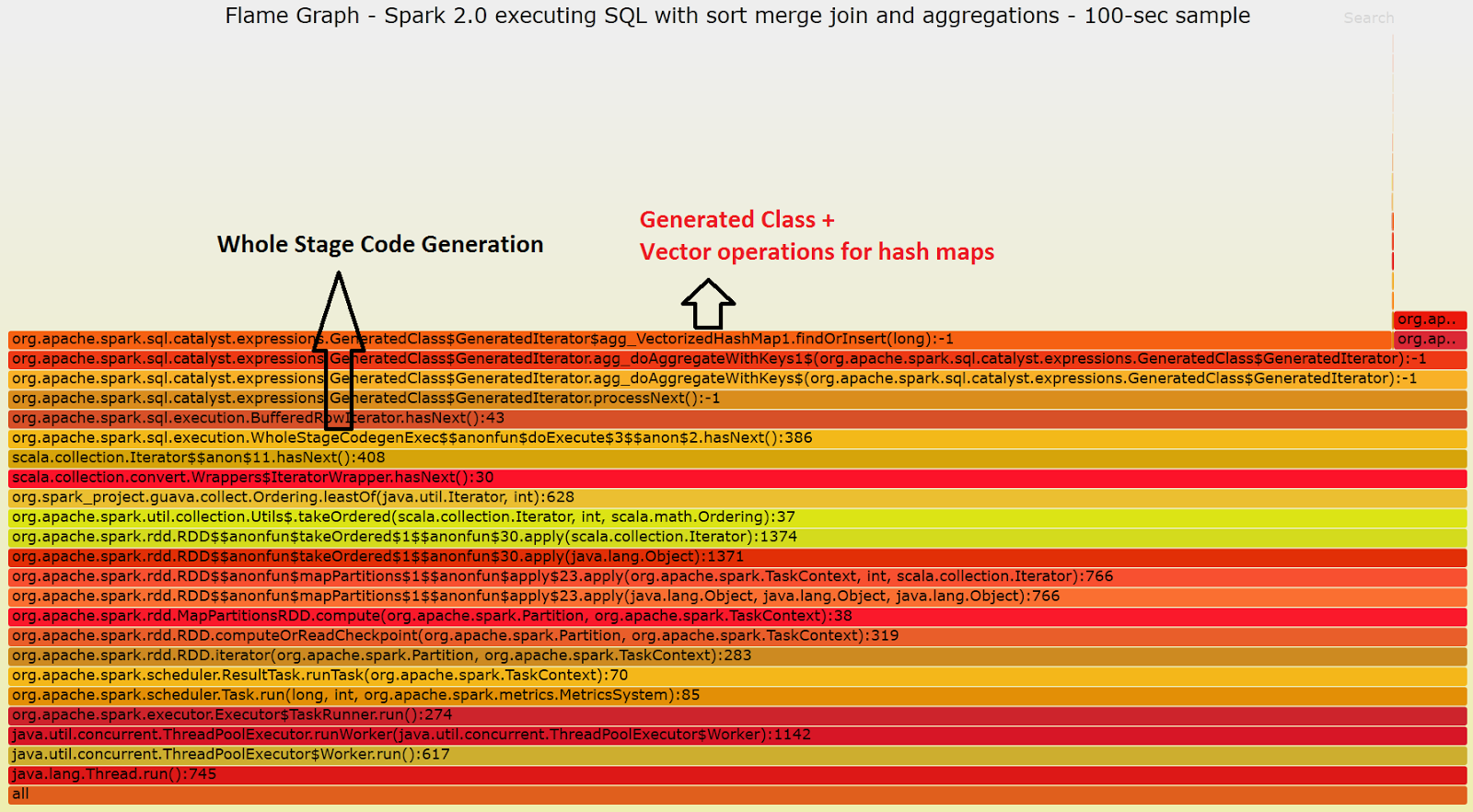
The test workload for this example is the one previously described in the post "Apache Spark 2.0 Performance Improvements Investigated With Flame Graphs". This is the code for preparing the test tables:

val testNumRows = 1e7.toLong
sql(s"select id from range($testNumRows)").createOrReplaceTempView("t0")
sql("select id, floor(200*rand()) bucket, floor(1000*rand()) val1, floor(10*rand()) val2 from t0").cache().createOrReplaceTempView("t1")
sql("select count(*) from t1").show

This part instantiates the classe used to measure Task metrics using custom listeners:

val taskMetrics = new ch.cern.sparkmeasure.TaskMetrics(spark)

This is the code to run the test workload:

taskMetrics.runAndMeasure(sql(
"select a.bucket, sum(a.val2) tot from t1 a, t1 b where a.bucket=b.bucket and a.val1+b.val1<1000 group by a.bucket order by a.bucket").show)

The metrics values collected and aggregated over all the tasks underlying the Spark workload under measurement (one SQL statement execution in this case) are:

Scheduling mode = FIFO
Spark Contex default degree of parallelism = 56
Aggregated Spark task metrics:
numtasks = 312
elapsedtime = 341393 (5.7 min)
sum(duration) = 10397845 (2.9 h)
sum(schedulerdelay) = 3737
sum(executorruntime) = 10353312 (2.9 h)
sum(executorcputime) = 10190371 (2.9 h)
sum(executordeserializetime) = 40691 (40 s)
sum(executordeserializecputime) = 8200 (8 s)
sum(resultserializationtime) = 105 (0.1 s)
sum(jvmgctime) = 21524 (21 s)
sum(shufflefetchwaittime) = 121732 (122 s)
sum(shufflewritetime) = 13101 (13 s)
sum(gettingresulttime) = 0 (0 ms)
max(resultsize) = 6305
sum(numupdatedblockstatuses) = 76
sum(diskbytesspilled) = 0
sum(memorybytesspilled) = 0
max(peakexecutionmemory) = 42467328
sum(recordsread) = 1120
sum(bytesread) = 74702928 (74.7 MB)
sum(recordswritten) = 0
sum(byteswritten) = 0
sum(shuffletotalbytesread) = 171852053 (171.8 MB)
sum(shuffletotalblocksfetched) = 13888
sum(shufflelocalblocksfetched) = 1076
sum(shuffleremoteblocksfetched) = 12812
sum(shufflebyteswritten) = 171852053 (171.8 MB)
sum(shufflerecordswritten) = 20769230

The main points to note from the output of the aggregated metrics are:

• The workload/SQL execution takes about 5 minutes of elapsed time (wall-clock time, as observed by the user launching the query). 
• The workload is CPU-bound: the reported values for "run time" and "CPU time" metrics are almost equal, moreover the reported values of other time-related metrics are close to 0 and negligible for this workload. This behavior was expected from the results of the analysis discussed at this link
• The total time spent executing the SQL summing the time spent by all the tasks is about 3 hours.
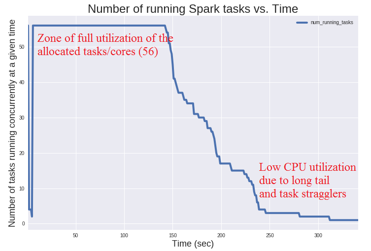
• The amount of CPU "cores" used concurrently, on average over the elapsed time of the SQL execution, can be estimated with this formula:   sum(executorcputime) / elapsedtime  = 10190371 / 341393 ~ 30
• The number of allocated cores by Spark executors is 56 (see also the reported value of default parallelism). Compare the 56 allocated cores to the calculated average CPU core utilization of 30. This points to the fact that the allocated CPUs were not fully utilized on average and it's worth additional investigations (more about this in the following)

Workload metrics show that the execution was CPU-bound but also that not all the potentially available CPU cycles on the executors were used. Why the low efficiency? The idea is to drill down on this performance-related question using the metrics collected by the TaskMetrics class and TaskInfoRecorderListener, which detail the behavior of each executed task. As a reference, the following piece of code can be used to export all the collected metrics into a DataFrame and also to save them to a file for further analysis:

// export task metrics information into a Spark DataFrame for analysis 
// if needed, also save them to disk

val df = taskMetrics.createTaskMetricsDF()

taskMetrics.saveData(df, "myPerfTaskMetrics1")

Note: It is also useful to note the start and end time of the execution of the code of interest. When using taskMetrics.runAndMeasure those values can be retrieve by printing taskMetrics.beginSnapshot and taskMetrics.endSnapshot, another option is to run System.currentTimeMillis() at the start and end of the workload of interest

The plot of the "Number of running Spark tasks vs. Time" (see below) can give you more clues on why the allocated CPUs were not fully ustilized during the workload execution. You can see that (1) in the first 150 seconds of the workload execution, the system uses all the available cores, after that it starts to slowly "ramp down", finally an important amount of time is spent on a long tail with some "straggler tasks". This provides additional information on why and how the SQL query under study was not able to use all the available CPUs all the time, as discussed above: we find that some of the available CPUs were idle for a considerable amount of time. It is worth reminding that this particular workload is CPU bound (i.e. no significant time is spent on I/O or other activities). For the pourpose of this post we can stop the analysis here. You can find the code for this analysis, with plots and additional drill down on the collected metrics in the notebook at this link

Why is this useful: Performing  analysis of the workload by drilling down into the metrics collected at the task level is of great help to understand why a given workload performs in a certain way and to identify the bottlenecks. The goal is also to derive actionable information to further improve the performance. You may be already familiar with investigating Spark performance using the Event Timeline in the  Spark WebUI, which already makes this type of investigations possible.
The techniques discussed in this post allow to extend and generalize the analysis, the idea is that you can export all the available metrics to your favorite analytics tool (for example a Jupyter notebook running PySpark) and experiment by aggregating and filtering metrics across multiple dimensions. Moreover the analysis can span multiple stages or jobs as needed and can correlate the behavior of all the collected metrics, as relevant (elapsed time, CPU, scheduler delay, shuffle I/O time, I/O time, etc). Another point is that having the metrics stored on a file allows to compare jobs performance across systems and/or application releases in a simple way and opens also the way to automation of data analysis tasks

Example 3:  This example is about measuring a complex query taken from the TPCS-DS benchmark at scale 1500GB deployed using spark-sql-perf. The query tested is TPCDS_v1.4_query 14a. The amount of I/O and of shuffle to support the join operations in this query are quite important. In this example Spark was run using 14 executors (on a cluster) and a total of 28 cores (2 cores for executor). Spark version: 2.1.0. The example is reported mostly to show that sparkMeasure can be used also for complex and long-running  workload. I postpone the analysis, as that would go beyond the scope of this post. The output metrics of the execution of query TPCDS 14a in the test environment described above are:

Scheduling mode = FIFO
SparkContex default degree of parallelism = 28
numstages = 23
sum(numtasks) = 13580
sum(duration) = 6136302 (1.7 h)
sum(executorruntime) = 54329000 (15.1 h)
sum(executorcputime) = 36956091 (10.3 h)
sum(executordeserializetime) = 52272 (52 s)
sum(executordeserializecputime) = 28390 (28 s)
sum(resultserializationtime) = 757 (0.8 s)
sum(jvmgctime) = 2774103 (46 min)
sum(shufflefetchwaittime) = 6802271 (1.9 h)
sum(shufflewritetime) = 4074881 (1.1 h)
max(resultsize) = 12327247
sum(numupdatedblockstatuses) = 894
sum(diskbytesspilled) = 0
sum(memorybytesspilled) = 1438044651520 (1438.0 GB)
max(peakexecutionmemory) = 379253665280
sum(recordsread) = 22063697280
sum(bytesread) = 446514239001 (446.5 GB)
sum(recordswritten) = 0
sum(byteswritten) = 0
sum(shuffletotalbytesread) = 845480329356 (845.5 GB)
sum(shuffletotalblocksfetched) = 1429271
sum(shufflelocalblocksfetched) = 104503
sum(shuffleremoteblocksfetched) = 1324768
sum(shufflebyteswritten) = 845478036776 (845.5 GB)
sum(shufflerecordswritten) = 11751384039

The flight recorder mode for sparkMeasure

  

Flight recorder mode addresses the cases when you need to instrument a Spark application but do not want (or cannot) add code to your job(s) to instantiate the custom listeners and attach them to the active Spark Context (for example using StageMetrics and/or TaskMetrics class, as was the case in the previous examples). You can deploy the metrics data collection in offline ("flight recorder") mode by adding custom listener code into Spark ListenerBus when starting the Spark Context.
For example using the spark-submit command line you can do that by adding: "--conf spark.extraListeners=...". The code for two listeners suitable for "Flight Mode" is provided with sparkMeasure: FlightRecorderStageMetrics and FlightRecorderTaskMetrics, respectively to measure stage- and task-level metrics. Example:

$ spark-submit --conf spark.extraListeners=ch.cern.sparkmeasure.FlightRecorderStageMetrics --packages ch.cern.sparkmeasure:spark-measure_2.11:0.11 ...additional jars and/or code

The flight recorder mode will save the results in serialized format on a file in the driver's filesystem. The action of saving the metrics to a file happens at the end of the application and is triggered by intercepting the relative event using the listener. Additional parameters are available to specify the name of the output files:

--conf spark.executorEnv.taskMetricsFileName=<file path> (defaults to "/tmp/taskMetrics.serialized")
--conf spark.executorEnv.stageMetricsFileName=<file path> (defaults to "/tmp/stageMetrics.serialized")

You will need to post-process the output files produced by the "Flight Recorder" mode. The reason is that the saved files contain the collected metrics in the form of serialized objects. You can read the files and deserialize the objects using the package Utils provided in sparkMeasure. After deserialization the values are stored in a ListBuffer that can be easily transformed in a DataFrame. An example of what all this means in practice:

val taskVals = ch.cern.sparkmeasure.Utils.readSerializedTaskMetrics("<file name>")
val taskMetricsDF = taskVals.toDF

Similarly, when post-processing stage metrics:
val stageVals = ch.cern.sparkmeasure.Utils.readSerializedStageMetrics("<file name>")
val stageMetricsDF = stageVals.toDF

Recap and main points on how and why to use sparkMeasure

• Use sparkMeasureto measure Spark workload performance. Compile and add the jar of sparkMeasure to your Spark environemnt
• Consider sparkMeasure as an alternative and extension of spark.time(<spark code>), instead just measuring the elapsed time with stageMetrics.runAndMeasure(<spark code>) or taskMetrics.runAndMeasure(<spark code>) you have the summary of multiple workload metrics
• Start with measuring at Stage level, as it is more lightweight. Use the Task-level metrics if you need to drill down on task execution details or skew (certain tasks or hosts may behave differtly than the average)
• Export metrics for offline analysis if needed and import them in your tool of choice (for example a notebook environment).

Summary and further work

    
Collecting and analyzing workload metrics beyond simple measurement of the elapsed time is important to drill down on performance investigations with root-cause analysis. sparkMeasure is a tool and proof-of-concept code that can help you collect and analyze workload metrics of Apache Spark jobs.
You can use sparkMeasure to investigate the performance of Spark workloads both for Scala and Python environments. You can use it from the command-line shell (REPL) or Jupyter notebook or as an aid to instrument your code with custom listeners and metrics reports. It is also possible to use sparkMeasure to collect and store metrics for offline analysis.
The available metrics are collected by extending the Spark listener interface, similarly to what is done by the Spark WebUI. The collected metrics are transformed into Spark DataFrames for ease of analysis.
sparkMeasure allows to collect metrics at the Task level for fine granularity and/or aggregated at Stage level. The collected metrics data come from existing Spark instrumentation. For the case of Spark 2.1.0 this includes execution time, CPU time, time for serialization and deserialization, shuffle read/write time, HDFS I/O metrics and others (see more details in sparkMeasure documentation and code). See also this example analysis of Task Metrics data using a notebook.

In this post you can find some simple examples of how and why to use sparkMeasure to drill down on performance metrics. Ideas for future work in this area include:

• add more examples to illustrate the meaning and accuracy of Spark instrumentation metrics
• show further examples where actionable info or insights can be gained by drilling down into Spark performance metrics
• show limitations of the currently available instrumentation (for example in the area of instrumentation for I/O service time)
• measure the overhead of the instrumentation using Spark listeners
• additional insights that can be derived by examining skew in the distribution of performance metrics at the task level

Acknowledgements

This work has been developed in the context of the CERN Hadoop and Spark service: credits go to my colleagues there for collaboration, in particular to Prasanth Kothuri and Zbigniew Baranowski. Thanks to Viktor Khristenko for direct collaboration on this topic and for his original work on the instrumentation of spark-root with Spark listeners.
Other material that has helped me for the development of this work are Jacek Laskowski's writeup and presentations on the subject of Spark Listeners and the presentation "Making Sense of Spark Performance" by Kay Ousterhout.
The Spark source code and the comments therein have also been very useful for researching this topic. In particular I would like to point to the Scheduler's code for the Spark Listener and the WebUI's JobProgressListener.

IPython/Jupyter SQL Magic Functions for PySpark

Topic: this post is about a simple implementation with examples of IPython custom magic functions for running SQL in Apache Spark using PySpark and Jupyter notebooks.

If you are already familiar with Apache Spark and Jupyter notebooks you may want to go directly to the example notebook and code. If you want additional context and introduction to the topic of using Spark on notebooks, please read on.

• Notebook with examples of %sql magic functions for PySpark
• Code of the example of IPython %sql magic functions 

Jupyter notebooks and Spark SQL

Notebooks are very useful and popular environments for data analysis. Among others they provide a user friendly environment for exploratory analysis and simplify the task of sharing your work such as preparing presentations and tutorials. Jupyter notebooks in particular are very popular, especially with Python users and data scientist. One of the neat tricks that you can do with IPython and Jupyter notebooks is to define "custom magic functions", these are commands processed by IPython that can be used as shortcuts for needed actions and functions. The custom magic functions extend the list of built-in magic commands.
In particular when running SQL in notebook environments, %sql magic functions provide handy shortcuts to the code. Custom magic functions come in two flavors, one is the line functions, such as %sql, that take their input from one line. For those cases where you want to run SQL statements that span over multiple lines you can use %%sql which works with cell input.
Apache Spark is a popular engine for data processing at scale. Spark SQL in particular provides a scalable and fast engine and API for processing structured data (see also docs in the references section of this post).
In this post you will find a simple way to implement magic functions for running SQL in Spark using PySpark (the Python API for Spark) with IPython and Jupyter notebooks.

IPython magic

One typical way to process and execute SQL in PySpark from the pyspark shell is by using the following syntax: sqlContext.sql("<SQL statement>") (code tested for pyspark versions 1.6 and 2.0) . It is easy to define %sql magic commands for IPython that are effectively wrappers/aliases that take the SQL statement as argument and feed them to sqlContext (see the docs at "custom magic functions"). An example of magic functions for running SQL in pyspark can be found at this link to the code . The following magic functions are defined in the accompanying example code:

%sql <statement>          - return a Spark DataFrame for lazy evaluation of the SQL
%sql_show <statement>     - run the SQL statement and show max_show_lines (50) lines 
%sql_display <statement>  - run the SQL statement and display the results using an HTML table. This is implemented passing via Pandas and displays up to max_show_lines (50)
%sql_explain <statement>  - display the execution plan of the SQL statement

An example of how the listed magic functions can be used to run SQL in PySpark can be found at this link to the example notebook. The code is simple and you can easily modify it to fit your needs, if different from the provided examples.

Tips on how build a test environment

If you are not familiar with using Spark SQL and notebooks, here some links that can help you get started.
Download Spark from http://spark.apache.org/downloads.html
Note: you will not need to have Hadoop and/or a YARN cluster installed to run the tests described in this post.
An easy way to install a Python environment and Jupyter is by downloading Anaconda from https://www.continuum.io/downloads
If not yet installed in your test machine, you can download Java 8 from Oracle Technet: http://www.oracle.com/technetwork/java/javase/downloads/index.html

The Python shell for Spark can be started simply by running "pyspark".
If you want to run pyspark inside a Jupyter notebook, as in the example notebook provided with this post, you can do that by setting the environment variable PYSPARK_DRIVER_PYTHON prior to running pyspark. Example:
export PYSPARK_DRIVER_PYTHON=$PATH_TO_ANACONDA/bin/jupyter-notebook

I also find this additional (optional) configuration useful:
export PYSPARK_DRIVER_PYTHON_OPTS="--ip=`hostname` --browser='/dev/null' --port=8888"

Similarly if you just want to run pyspark under IPython using the command line (rather than the web notebook interface with Jupyter), you can set PYSPARK_DRIVER_PYTHON to point to the executable for IPython prior to running pyspark. Example:
export PYSPARK_DRIVER_PYTHON=$PATH_TO_ANACONDA/bin/ipython

The paragraphs just lists a few examples of how you can get started with running the code described in this post. There are other ways to start your Python notebook environment for Spark. Notably you can start the notebook with IPython/Jupyter first and later manually start the Spark Context and SQLContext, therefore bypassing the use of the pyspark tool/shell.


Links to documentation, references and previous work

Link to Apache Spark documentation on Spark SQL and DataFrames and PySpark API.
Spark SQL Language Manual, which is part of the Databricks User Guide.
Overview article on Spark: "Apache Spark: A Unified Engine for Big Data Processing" in Communications of the ACM November 2016.
Article with details on Spark SQL: "Spark SQL: Relational Data Processing in Spark", proceeding of SIGMOD 2015
I have covered in this blog other examples of how to implement and use %sql magic functions, see: "IPython/Jupyter Notebooks for Oracle" and "IPython Notebooks for Querying Apache Impala".
Previous work published in this blog on Spark SQL includes "Apache Spark 2.0 Performance Improvements Investigated With Flame Graphs".
This blog post and accompanying example code have been developed in the context of the CERN IT Hadoop and Spark service.

Apache Spark 2.0 Performance Improvements Investigated With Flame Graphs

Topic: This post is about performance optimizations introduced in Apache Spark 2.0, in particular whole-stage code generation. A test case is introduced and investigated with diagnostic tools.


Introduction: performance troubleshooting of a slow query using parallel query execution in a Hadoop cluster

The idea for this post comes from a performance troubleshooting case that has come up recently at CERN database services. It started with a user reporting slow response time from a query for a custom report in a relational database. After investigations and initial troubleshooting, the query was still running slow (running in about 12 hours). It was understood that the query was mostly running "on CPU" and spending most of its time in evaluating a non-equijoin condition repeated 100s of millions of times. Most importantly it was also found that the query was easily parallelizable, this was good news as it meant that we could simply "throw hardware at it" to make it run faster. One way that the team (see the acknowledgments section at the end of the post) used to parallelize the workload (without affecting the production database), is to export the data to a Hadoop cluster and run the query there using Spark SQL (the cluster used has 14 nodes, installed with CDH 5.7, Spark version 1.6). This way it was possible to bring the execution time down to less than 20 minutes. All this with relatively low effort, as the query could be run basically unchanged.
This post is about Spark, however it is interesting to note that the query was also tested using Apache Impala (version 2.5) on the same cluster and produced comparable speedup results. Later I have also run the query on a "beefy Oracle server" with 60 cores adding the relevant configuration for activating Oracle parallel query (test done on Oracle RDBMS version 12.1.0.2) reproducing comparable execution times/speedup as in the cases of Spark and Impala.


Spark 2.0 enters the scene

As I write this post, Spark 1.6 is installed in our production clusters and Spark 2.0 is still relatively new (it has been released at the end of July 2016). Notably Spark 2.0 has very interesting improvements over the previous versions, among others improvements in the area of performance that I was eager to test (see this blog post by Databricks).
My first test was to try the query discussed in the previous paragraph on a test server with Spark 2.0 and I found that it was running considerably faster than in the tests with Spark 1.6. The best result I achieved, this time on a large box with 60 CPU cores and using Spark 2.0, was an elapsed time of about 2 minutes (to be compared with 20 minutes in Spark 1.6). I was impressed by Spark 2.0's speedup compared to Spark 1.6 and decided to investigate further.


The test case

Rather than using the original query and data, I will report here on a synthetic test case that hopefully illustrates the main points of the original case and at the same is simple and easy to reproduce on your test systems, if you wish to do so. This test uses pyspark, the Python interface to Spark, in the simplest configuration for a test machine: local mode (that is without hadoop or yarn). If needed you can add to the command line "--master local". If you are not familiar with how to run Spark, see further on in this post some hints on how to build a test system.

The preparation of the test data proceeds as follows: (1) it creates a DataFrame and registers it as table "t0" with 10 million rows. (2) Table t0 is used to create the actual test data, which is composed of an "id" column and three additional columns of randomly generated data, all integers. The resulting DataFrame is cached in memory and "registered" as a temporary table called "t1". Spark SQL interface for DataFrames makes this preparation task straightforward:

$ pyspark --driver-memory 2g

test_numrows = 1e7

sqlContext.range(0,test_numrows,1).registerTempTable("t0")

sqlContext.sql("select id, floor(200*rand()) bucket, floor(1000*rand()) val1, floor(10*rand()) val2 from t0").cache().registerTempTable("t1")

The following commands are additional checks to make sure the table t1 has been created correctly and is first read into memory. In particular, note that "t1" has the required test_numrows (10M) rows and the description of its column from the output of the command "desc":

sqlContext.sql("select count(*) from t1").show()

+--------+
|count(1)|
+--------+
|10000000|
+--------+

sqlContext.sql("desc t1").show()

+--------+---------+-------+
|col_name|data_type|comment|
+--------+---------+-------+
|      id|   bigint|       |
|  bucket|   bigint|       |
|    val1|   bigint|       |
|    val2|   bigint|       |
+--------+---------+-------+

The actual test query is here below. It consists of a join with two conditions: an equality predicate on the column bucket, which becomes an obvious point of where the query can be executed in parallel, and a more resource-intensive non-equality condition. Notably the query has also an aggregation operation. Some additional boilerplate code is added for timing the duration of the query:

import time
starttime=time.time()

sqlContext.sql("select a.bucket, sum(a.val2) tot from t1 a, t1 b where a.bucket=b.bucket and a.val1+b.val1<1000 group by a.bucket order by a.bucket").show()

print("Delta time = %f" % (time.time()-starttime))

The results are that Spark 2.0 is about 7 times faster than Spark 1.6 when running the test query on the test server (see details below): Spark 2.0 completed the job in about 15 minutes of elapsed time and 390 minutes of CPU time, while Spark 1.6 took about 100 minutes of elapsed time and 2840 minutes of CPU time. There are fluctuations on the actual job execution time between runs, however you can ignore the fine details and focus on the main finding that the performance difference is striking between runs using Spark 1.6 and Spark 2.0 (Spark 2.0 being much faster). This is worth further investigations into the internals and root causes.

I have run the tests using Spark in its simplest configuration (local mode) using a standalone (non-clustered) server with 16 cores (2 x  E5-2650) and 128 GB of RAM (the virtual memory allocated by the test workload is about 16 GB) running Linux (kernel 2.6.32, RHEL 6.7). If you want to run it on a smaller machine you can scale down the preparation phase by setting test_numrows to a smaller value (for example to 1e6). In that case you probably could do also with using the default value of 1g for the driver-memory.
The tests have been performed on a single server alternating runs with Spark 1.6 and 2.0. In both cases monitoring with OS tools showed that the jobs were CPU-bound, that is with 32 threads (16 cores x 2 for multithreading) running on CPU and utilizing the available resources on the test box. During the tests, no additional significant workload was running on the box.


Drilling down into the execution plans

The physical execution plan generated and executed by Spark (in particular by Catalyst, the optimizer and Tungsten, the execution engine) has important differences in Spark 2.0 compared to Spark 1.6. The logical plan for executing the query however deploys a sort merge join in both cases. Please note in the execution plans reported here that in the case of Spark 2.0 several steps in the execution plan are marked with a star (*) around them. This marks steps optimized with whole-stage code generation.


Physical execution plan in Spark 1.6:

Note that a sort merge join operation is central to the execution plan of this query. Another important step after the join is the aggregation operation, used to compute "sum(a.val2)" as seen in the query text:

Physical execution plan in Spark 2.0:

Note in particular the steps marked with (*), they are optimized with who-stage code generation:

Details of the SQL execution from the Spark Web UI, Spark 1.6. vs. Spark 2.0. This reproduces the physical execution plan with additional metrics gathered at run-time. Note in particular in Spark 2.0 the steps marked as "Whole Stage Codegen".

Code generation is the key

The key to understand the improved performance is with the new features in Spark 2.0 for whole-stage code generation. This is expected and detailed for example in the blog post by Databricks Engineering "Apache Spark as a Compiler: Joining a Billion Rows per Second on a Laptop Deep dive into the new Tungsten execution engine". The main point is that Spark 2.0 compiles query execution into bytecode that is then executed, as opposed to looping with an iterator over result sets. A detailed discussion on the benefits of query compilation and code generation vs. the "traditional approach" to query execution, also called volcano model, can be found in the lecture by Andy Pavlo on Query Compilation.

Run time investigations with flame graphs

Flame graphs visualization of stack profiles provide additional insights on which parts of the code are executed and where CPU cycles are consumed. The upper layers of the flame graph highlight where CPU cycles are spent. The lower layers add context by detailing the information on the parent functions/methods that called the "upper layers". The idea for this paragraph is to use stack profiles and flame graphs to further drill down on the differences in the execution model between Spark 2.0 and Spark 1.6.

To collect and generate the flame graphs I have used the methods described by Kay Ousterhout in "Generating Flame Graphs for Apache Spark using Java Flight Recorder".  I have used the Java flight recorder on Oracle's Java 8, starting pyspark with the following options:

pyspark --conf "spark.driver.extraJavaOptions"="-XX:+UnlockCommercialFeatures -XX:+FlightRecorder" --conf "spark.executor.extraJavaOptions"="-XX:+UnlockCommercialFeatures -XX:+FlightRecorder"

Note added October 2017: see this link for more info on tools and techniques available for stack profiling and flame graph visualization for Spark.

Here below you can find two flame graphs that visualize the stack profiles collected for Spark 1.6 and Spark 2.0 while running the test workload/query. The graphs represent samples collected over 100 seconds. The major differences you should notice between the two flame graphs are that on Spark 1.6 the execution iterates over rows of data, looping on Row Iterator to Scala for example. In the Spark 2.0 example, however, you can see in the flame graph that the methods executing the bulk of the work are built/optimized with whole-stage code generation. For example the method where most time is spent during execution is code-generated and performs operations on Hash Maps in vector form.

What you can learn from flame graphs:

• The flame graph for Spark 1.6 shows that a considerable amount of CPU cycles are spent on the Scala collection iterator. This can be linked with Spark 1.6 using the "traditional volcano model" for SQL execution. This is the part that is optimized in Spark 2.0 (see next bullet points).
• Spark 2.0 is making use of whole-stage code generation and does not use Scala collection iterator.
• Spark 2.0 is also using Vectorized Hash Maps to perform aggregations that are also code generated. The use of vectorized operations is likely introducing further performance improvements.

Spark 1.6:

Flame graph for a sample of the execution of the test query using Spark 1.6 in local mode (on a machine with 16 cores). Note that most of the time is spent processing data on a iterative way (which is not optimal). Click on this link for a SVG version of the graph where you can drill down on the details of each step.


Spark 2.0:

Flame graph for a sample of the execution of the test query using Spark 2.0 in local mode (on a machine with 16 cores). Note that most of the time is spent executing code that is generated dynamically via whole-stage code generation. Click on this link for a SVG version of the graph where you can drill down on the details of each step.


Note: the process of collecting stack profiles for Spark in this test is made easier by the fact that I have used Spark in local mode, which results in only one (multi-threaded) process to trace in a single box . In the general case tracing Spark is more complicated due to the distributed nature of the workload when running on a cluster for example.


Linux Perf stat counters

In this paragraph you can find the output of Linux Perf stat counters measured during the execution of the test query. The idea is to find differences in the run-time usage of resources that can further highlight the origin of the performance improvement that was measured in Spark 2.0 compared to Spark 1.6. The selection of stat counters to measure is taken from Tanel Poder's blog post "RAM is the new disk – and how to measure its performance – Part 2 – Tools". Notably you can find there also a short explanation of meaning of the counters.

# perf stat -e task-clock,cycles,instructions,branches,branch-misses \
          -e stalled-cycles-frontend,stalled-cycles-backend \
          -e cache-references,cache-misses \
          -e LLC-loads,LLC-load-misses,LLC-stores,LLC-store-misses \
          -e L1-dcache-loads,L1-dcache-load-misses,L1-dcache-stores,L1-dcache-store-misses \
          -p <pid_spark_process> sleep 100

What you can learn from comparing perf stat counters between Spark 1.6 and Spark 2.0 runs:

• In both cases the workload is CPU-bound. The machine has 16 cores and is configured with multi-threading support (i.e. 32 execution threads). Perf stat counters report an average CPU utilization of about 31 CPU threads in both cases, which confirms the fact that the workload is CPU bound.
• Reading from main memory seems to be key and Spark 2.0 appears to access memory with much higher throughput than Spark 1.6. In particular, I believe it is important to look at the counters LLC-loads and LLC-load-misses, those count respectively how many time a cache line was requested from last level cache (LLC) and the fraction of those requests that resulted in access from main memory. Notably Spark 2.0 in the given sample reports 33 M/sec LLC-loads with ~63% of loads resulting in misses (reads from main memory) while Spark 1.6 has 0,7 M/sec LLC-loads and also ~60% misses. I have noticed that these values fluctuate over different samples, but Spark 2.0 presents always much higher access rate to LLC and memory than Spark 1.6.
• It is interesting to note that the measurements in the case of Spark 1.6 run present a higher ratio of instructions per cycle than the run with Spark 2.0. Spark 2.0 workload is stalling for memory access more frequently. A higher ratio of instructions per cycle is often an indicator of better performance, however, in this case the opposite appears to be true. I believe a possible interpretation of what is happening is that Spark 2.0 is more efficient at using CPU resources and high throughput to memory, therefore it quickly gets into what appears to be the bottleneck for this workload: stalling for memory access.

This is the output of perf stat while running the test workload with Spark 1.6:

    3091790.707578      task-clock (msec)         #   30.915 CPUs utilized
 7,325,423,029,717      cycles                    #    2.369 GHz                     [25.01%]
 9,577,944,921,957      instructions              #    1.31  insns per cycle
                                                  #    0.45  stalled cycles per insn [31.25%]
 1,323,763,955,367      branches                  #  428.154 M/sec                   [31.06%]
     3,540,000,205      branch-misses             #    0.27% of all branches         [25.02%]
 4,332,575,248,710      stalled-cycles-frontend   #   59.14% frontend cycles idle    [25.02%]
 1,809,219,108,190      stalled-cycles-backend    #   24.70% backend  cycles idle    [25.01%]
     4,025,591,940      cache-references          #    1.302 M/sec                   [27.12%]
     2,688,865,386      cache-misses              #   66.794 % of all cache refs     [29.14%]
     2,305,317,283      LLC-loads                 #    0.746 M/sec                   [25.40%]
     1,382,318,864      LLC-load-misses           #   59.96% of all LL-cache hits    [25.40%]
     1,265,162,587      LLC-stores                #    0.409 M/sec                   [24.60%]
     1,256,986,002      LLC-store-misses          #    0.407 M/sec                   [26.51%]
 3,084,754,630,344      L1-dcache-loads           #  997.724 M/sec                   [29.69%]
    18,141,140,551      L1-dcache-load-misses     #    0.59% of all L1-dcache hits   [28.93%]
   891,386,721,821      L1-dcache-stores          #  288.308 M/sec                   [25.97%]
     1,281,601,143      L1-dcache-store-misses    #    0.415 M/sec                   [25.20%]

This is the output of perf stat while running the test workload with Spark 2.0:

    3095743.023060      task-clock (msec)         #   30.955 CPUs utilized
 7,267,137,941,598      cycles                    #    2.347 GHz                     [25.01%]
 5,810,442,547,610      instructions              #    0.80  insns per cycle
                                                  #    1.00  stalled cycles per insn [31.25%]
 1,142,058,628,367      branches                  #  368.913 M/sec                   [31.07%]
    17,683,392,720      branch-misses             #    1.55% of all branches         [25.43%]
 5,791,745,210,259      stalled-cycles-frontend   #   79.70% frontend cycles idle    [25.23%]
 3,993,653,110,520      stalled-cycles-backend    #   54.95% backend  cycles idle    [25.03%]
    51,936,035,185      cache-references          #   16.777 M/sec                   [30.84%]
    14,525,498,107      cache-misses              #   27.968 % of all cache refs     [25.21%]
   104,521,878,980      LLC-loads                 #   33.763 M/sec                   [25.01%]
    66,262,327,528      LLC-load-misses           #   63.40% of all LL-cache hits    [28.30%]
       301,797,039      LLC-stores                #    0.097 M/sec                   [26.72%]
       215,020,365      LLC-store-misses          #    0.069 M/sec                   [24.58%]
 2,520,703,012,324      L1-dcache-loads           #  814.248 M/sec                   [24.80%]
    96,261,558,827      L1-dcache-load-misses     #    3.82% of all L1-dcache hits   [24.99%]
   178,644,475,917      L1-dcache-stores          #   57.706 M/sec                   [29.09%]
     1,045,403,531      L1-dcache-store-misses    #    0.338 M/sec                   [27.73%]

Source code

If you want to further drill down on the changes  in Spark 2.0 that benefit the performance of the test workload you can head to GitHub and browse the source code of Spark. For example from the flame graphs you can find the name of relevant the classes with path and/or you can use the search function in GitHub. So far I have only skimmed through the source code with these methods and found a few links that I believe are interesting as an example of the drill-down analysis that one can do thanks to the fact that Spark is an open source project:

• One link of interest is "org.apache.sql.execution.WholeStageCodegenExec". This is code introduced in the Spark 2.0 branch, you can find there also comments that shed some light on the mechanism used for code generation.
• Another interesting point is about the use of "vectorized hash maps" in Spark 2.0, which appears important as it is on the top line of the Spark 2.0 flame graph: "org.apache.spark.sql.executio.aggregate.VectorizedHashMapGenerator.scala" has additional details about the implementation. You can find there that this is an implementation for fast index lookup, also introduced in the Spark 2.0 branch. It is also mentioned there that the execution can be code generated for boosting its performance, that is what you can see happening in the flame graph of Spark 2.0 workload.

Tips on how to build a test environment 

For the readers who are not familiar with running Spark, here some tips on how to build a test environment:
Download Spark from http://spark.apache.org/downloads.html
You will not need to have Hadoop and/or a YARN cluster to run the tests described in this post.
An easy way to install a Python environment is by downloading Anaconda from https://www.continuum.io/downloads
You can download Java 8 from Oracle technet: http://www.oracle.com/technetwork/java/javase/downloads/index.html
Code for generating flame graphs for Spark using Java Flight Recorder (see the recipe at this link) at: https://github.com/brendangregg/FlameGraph and https://github.com/chrishantha/jfr-flame-graph

Summary

Apache Spark 2.0 has important optimizations for performance compared to Spark version 1.6. Notably Spark optimizer and execution engine in version 2.0 can take advantage of whole-stage code generation and of vector operations to make more efficient use of CPU cycles and memory bandwidth for improved performance. This post briefly discusses an example how Spark SQL and its parallel execution engine have been useful to tune a query from a production RDBMS. Moreover an example comparing Spark 1.6 and Spark 2.0 performance has been discussed and drilled-down using execution plan details, flame graphs and Linux Perf stat counters.


Additional comments and my take-away from the tests in this post

The Hadoop ecosystem provides a powerful and easy-to-use environment for running reports and analytics queries. The point is nicely illustrated for me by the fact that we could simply take data and a query from production RDBMS and run it on the Hadoop cluster (with Spark and Impala) to make it run with parallelism and fast. This provides a simple and quick way to throw HW at a performance problem.

I am impressed by the work on Spark 2.0 optimizations for whole-stage code generation, in particular by how these new features address the important point of how to optimize CPU-bound workloads.  This makes a great addition to Spark and strengthen its position as a leading player in data processing a scale.

Query compilation and/or code generation for executing SQL has become a common feature for many of the new databases appearing on the market optimized for "in memory" (i.e. processing an important fraction of their workload in main memory). This is implemented in various forms for different products, however it is proven to give significant gains in performance, typically of the order of one order of magnitude, for queries where it is applicable. The test case examined in this post provides an example of this type of optimization.

How are the mainstream RDBMS engines, that typically process result sets in an iterative way (similarly to what was found in this post with Spark 1,6 and often referred to as the volcano model) going to respond to this performance-based challenge?


Acknowledgements and references

This work has been made possible and funded by CERN IT, in particular in the context of the CERN IT Hadoop Service and Database Services. In particular I would like to thanks CERN colleagues who have contributed to the performance troubleshooting case mentioned in this post: Raul Garcia Martinez, Zbigniew Baranowski and Luca Menichetti.

On the topic of Spark 2.0 improvements for code generation, see the blog post "Apache Spark as a Compiler: Joining a Billion Rows per Second on a Laptop" and the references therein, notably including "Efficiently compiling efficient query plans for modern hardware" and JIRA ticket SPARK-12795.

On flame graphs for Spark: Kay Ousterhout in "Generating Flame Graphs for Apache Spark using Java Flight Recorder". See also "Hadoop performance troubleshooting with stack tracing, an introduction".

On the topic of query compilation on modern database systems vs. the volcano model, see also the lecture by Andy Pavlo on Query Compilation.
Flame graphs are the brain child of Brendan Gregg.
Additional links on using Linux Perf to measure performance counters: this article by Brendan Gregg and the 3-part blog posts by Tanel Poder on "RAM is the new disk".
On the topic of connecting Hadoop and relational databases see also Tanel's presentation "Connecting Hadoop and Oracle".