Wait Event History Sampling, an Experiment in Oracle Performance Analysis

Topic: This post is about a performance analysis technique based on high frequency sampling of wait event history data in Oracle. Two scripts are provided for performing this type of analysis and two example cases are discussed applied to the study random read latency and read workload characterization.

Context: In the context of performance analysis, for example for a study of I/O response time, I want to analyze the flow of all wait events for 'db file sequential read', say for a group of sessions. What are the options?

• 10046 trace is the classic way. This provides all the details of the SQL execution including wait event details if I want to. One of the problem here is with the scalability of writing into trace files especially if I want to trace many and very active sessions, in addition possibly tracing for a long time. Moreover the amount of data in the traces is an overkill for what I need, as I am interested only in some particular aggregations of db file sequential read wait events.
• DTrace of Oracle sessions provides an elegant and direct way to tap into the wait event interface for real-time analysis (see this article for details). However this method is still niche and works best in Solaris, while I mostly work with Oracle on Linux.
• Sampling is a typical alternative to tracing. Oracle ASH does just that and is a great source of performance data. However Oracle ASH data is sampled at 1 Hz, too slow for capturing I/O events. (Note: ASH sampling rate can be increased by tweaking _ash_sampling_interval, although the highest available rate currently is 10 Hz, still too low for our purposes).

Sampling of wait event history data

Oracle's V$SESSION_WAIT_HISTORY provides details of the last 10 wait events for each session currently connected to the instance. The idea is to use this data as a series of ring buffers, indexed by Oracle's SIDs. How can we wrap around the buffers? It turns out that the underlying X$KSLWH table has a column that can be used just for that: KSLWHWAITID (the values in KSLWHWAITID are not reported in V$SESSION_WAIT_HISTORY unfortunately). Here below an example of some of the columns of interest in X$KSLWH:

KSLWHSID	KSLWHWAITID	KSLWHETEXT	KSLWHETIME	KSLWHP1	KSLWHP2	KSLWHP3
42	21016	db file sequential read	300	25	148935	1
42	21015	db file sequential read	1020	25	47683	1
42	21014	db file sequential read	16024	25	124765	1
42	21013	db file sequential read	4100	25	57668	1

Example 1: fine-grained wait event latency histograms 

Let's put our sampling technique at work for capturing latency data and then display the collected data with latency histograms. Note: latency histograms and their graphical representations are useful for studies of random read performance, see also this previous article on the subject.

The advantage of the method based on sampling X$KSLWH over the use of  V$EVENT_HISTOGRAM are:

• The lowest bucket in V$EVENT_HISTOGRAM is 1 ms, which is too coarse for I/O coming from SSDs. By sampling we can reach to a finer scale (depending on the sampling rate, in practice ~100 micro seconds is easily reachable).
• We can apply a finer grain selection to the sessions we want to investigate, for example by limiting our sampling to one session or a group of sessions, as opposed to measuring the entire instance.

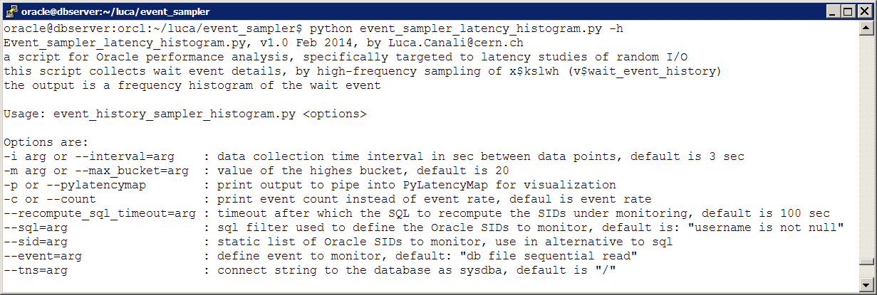
The tool: event_history_sampler_histogram.py is a python script that I wrote for this type of analysis. The script works by sampling X$KSLWH in a tight loop (which also mean it is CPU hungry). Here is a screenshot of the usage of this script with its options:

Here an example of the tool in actions with its output:

This script can be easily interfaced with PylatencyMap for heat map visualization. Here below is an example applied to displaying latency data of a workload generated with SLOB (note that the latency measurements are in microseconds):

$ python event_sampler_latency_histogram.py --sql="username like 'USER%'"|python ../PyLatencyMap/LatencyMap.py

Example 2: real-time analysis of all I/O instrumented by db file sequential read 

The use case here is to analyze all the I/O performed via db file sequential read and perform real-time analysis of the data. This is similar to the case above but instead of limiting the analysis to the latency time we want also to make use of the information on which blocks have been read.
For example we can record all the blocks that have been read and instrumented using db file sequential read in addition to their latency details. Details of the block read are available as wait event parameters p1 and p2 (file number and block number respectively). We can collect the data using a technique similar to what was described above for the latency histograms example: that is by sampling X$KSLWH.

Some examples of what can we learn from this type analysis:

• We can collect the list of all the blocks read in a given time interval. One of the simplest analysis is to count how may distinct blocks we have read. This gives an indication of how big the active area of the data set is for this workload. 
• We can use the information on the size of the active data set as help for sizing the cache (for example for sizing the needs for SSD cache in the storage, or sizing the amount of RAM needed for efficiently buffer the workload).
• We can study physical IO based on latency, for example by measuring how much of the workload is reading 'new blocks' or instead reading multiple times the same set of data blocks.
• In the example below you can see that for each sampling interval (the default is a 10-second interval) we have info on:
• the number of distinct blocks sampled since the script has started collecting 
• the number of blocks read during the latest collection interval having a latency <2 ms (presumably from SSD cache) and the drill-down details of whether they are new block reads or blocks that have been read before during sampling
• same as above but for blocks read with latency >=2 ms (presumably I/O coming from spindles) 
• It's also straightforward to add custom analysis code in the python script to provide for different use case, if needs arise.

Here below an example screenshot of test analysis performed with a python script I wrote called event_sampler_gather_IO_history.py:

$ python event_sampler_gather_IO_history.py --sql="username='MY_APP_USER'"

Limitations and additional comments

The main limitation of this method lies in the necessity to sample at high frequency, the higher the frequency the more events with low latency we can capture. In practice a frequency of 1 KHz seems good enough for the study of random reads. However this also means running the script in a 'tight loop' and consuming 1 core of CPU constantly during the execution of the script.
Moreover the execution time of the sampling query depends on the number of sessions monitored, therefore we will see lowering sampling rates as we increase the number of sampled sessions. In practice sampling up to a few hundred concurrent sessions at a time seems to give still good results.
Another limitation is due to the fact that we are only sampling db file sequential read waits and ignoring other wait events such as db file parallel read or in general multi-block and/or async IO events.
The script event_sampler_gather_IO_history.py works by collecting information on all blocks read during its execution. In the example above where information of 12M blocks was stored in a python dictionary, almost 2GB of RAM were used. The memory footprint of the script should be optimized in a future version, in the mean time memory consumption needs to be monitored when running this type of analysis.
Note for RAC: these scripts will only monitor activity in the instance where they are connecting to (basically it's like using V$ views as opposed to GV$).

Download the scripts:

The scripts mentioned in this blog are available from http://cern.ch/canali/resources.htm

Feel free to download and try them out, however beware that they are still in a beta stage.

The scripts have been tested against Oracle 11.2.0.3, 11.2.04 and 12.1.0.1 on Linux RHEL5 and RHEL6 with Python 2.4 and 2.6 and cx_Oracle version 5.1.2.

Conclusions

This article describes the main ideas of a technique for performance analysis of Oracle wait event data based on sampling the wait event history data and in particular X$KSLWH to produce a wait event data stream for real-time analysis. This has been illustrated with two examples related to to the study of random read latency and to the study of random IO patterns. The scripts used for this analysis are written in python and available for free download.

Clusterware 12c and Restricted Service Registration for RAC

Topic: This post is about exploring the mechanisms used by Oracle Clusterware 12.1.0.1 to restrict remote service registration, i.e. the 12c new feature "Restricting Service Registration for Oracle RAC Deployments"

Why is this useful? This improvement of 12c clusterware and listeners over the 11.2 version is useful mainly for security purposes, for example as a measure against TNS poisoning attacks (see also CVE-2012-1675), and it is particularly relevant for RAC deployments. Another important point is that it makes the DBA job easier by avoiding the complexity of COST (Class of Secure Transport) configurations (see also support Doc ID 1453883.1).
Notably Oracle 11.2 databases can profit of this 12c improvement too (in the case where the 11g RAC database installed under 12c clusterware).

Spoiler: If you have heard already about the 12c new feature of valid node checking for registration (VNCR) you are still in for a surprise.

Listeners in Oracle RAC in 11.2 and 12.1:
There have been important changes on how listeners are used in RAC starting with the clusterware 11.2. The details are discussed in a previous post. The main points are that (1) we now have local listeners and scan listeners, all using the same binary tnslsnr but with different scope. (2) Most of the listener configuration parameters, in RAC, are taken care of by the clusterware (Oraagent).
Database instances will perform remote service registration to remote listeners as specified by the instance parameter remote_listener (BTW remote service registration is needed to enable the server-side load balancing mechanism of RAC). PMON takes care of the registration in versions up to 11.2, in 12c a new LREG process has been introduced. Local service registration is configured at the instance level using the parmeter local_listener. Normally we will leave its value unset and the clusterware (Oraagent) will take care of setting it to the address of the local listener.  In 11.2 and higher the parameter listener_networks is also relevant, typically in the case of setups with more than one public network (the details are outside the scope of this discussion).

Why restricting service registration?
If service registration is not restricted, anybody who can reach the listener via the network can register a service with it. This opens the way to abuses, such as crafting an attack aimed at redirecting legitimate TNS traffic towards the attacker's machine (see also TNS poisoning attack mentioned above).

What's new in 12.1.0.1?
After performing a 12.1.0.1 vanilla RAC installation we notice that the scan listeners will only accept remote registration over TCP from local cluster nodes. This is an improvement over 11g where to obtain the same result the DBA had to manually execute a series of steps for COST (Class of Secure Transport) configuration, in order to configre the TCPS protocol to restrict remote registration. This improvement is listed as a new feature of 12c for RAC as "Restricting Service Registration for Oracle RAC Deployments".

How does 12c restrict service registration?
In $GRID_HOME/network/admin we can examine listener.ora: we notice a few additional lines from the equivalent file in version 11.2 (see also this post for more details on listener.ora in 11.2), that is lines containing valid node checking configuration. For example:

VALID_NODE_CHECKING_REGISTRATION_LISTENER=SUBNET # line added by Agent
VALID_NODE_CHECKING_REGISTRATION_LISTENER_SCAN1=OFF # line added by Agent

VALID_NODE_CHECKING_REGISTRATION_LISTENER_SCAN2=OFF # line added by Agent

With the first of those lines listed here above the clusterware (OraAgent), which takes care of most of the listener configurations, informs us that after starting the listener it has also connected to it (via IPC) and activated the new feature of valid node checking for registration (VNCR) for the listener called LISTENER, that is for the local listener.
What VNCR does is to restrict remote service registration, in this case to the local subnets.  A short recap for the possible values for the VNCR from support Note Id 1592571.1 is listed here below. See documentation for further details.

• OFF/0 - Disable VNCR
• ON/1/LOCAL - The default. Enable VNCR. All local machine IPs can register.
• SUBNET/2 - All machines in the subnet are allowed registration. This is for RAC installations.

What about the scan listener?
From the snippet of listener.ora reported above we can also see that VNCR is surprisingly turned OFF for the scan listeners (at least in this configuration that I have obtained after a vanilla 12.1.0.1 clusterware installation). However, as we can easily check (see more on techniques below) remote service registration to the scan listeners is indeed restricted and not possible for servers outside the RAC cluster. Therefore another mechanism, different from VNCR, is in place for scan listeners. Let's investigate!

Some explanations:
It turns out that the clusterware (OraAgent) does again the work, but this time without making it visible with an entry it in listener.ora. OraAgent takes care of setting the parameter REMOTE_REGISTRATION_ADDRESS for the scan listener, setting a endpoint for it on the HAIP network. Note, for more info on HAIP see documentation and support Doc Id 1210883.1
A log of this listener parameter change can be found in the logfile of the Clusterware Agent (OraAgent for crsd): $GRID_HOME/{NODE_NAME}/agent/crsd/oraagent_oracle/oraagent_oracle.log). The result can also be observed by using lsnrctl:

$ lsnrctl show remote_registration_address dbserver1-s:1521

Connecting to (DESCRIPTION=(CONNECT_DATA=(SERVICE_NAME=))(ADDRESS=(PROTOCOL=TCP)(HOST=xx.xx.xx.xx)(PORT=1521)))
dbserver1-s:1521 parameter "remote_registration_address" set to (DESCRIPTION=(ASYNC_TIMER=yes)(EXPIRE_TIME=1)(TRANSPORT_CONNECT_TIMEOUT=15)(ADDRESS_LISTDRESS=(PROTOCOL=tcp)(HOST=169.254.163.245)(PORT=11055))))

What does REMOTE_REGISTRATION_ADDRESS do?
When the listener receives a remote registration request it will reply to the client (which would normally be Oracle's PMON or LREG process) with a request to re-send the registration message via the HAIP network, in the example above: (HOST=169.254.163.245)(PORT=11055). This would only be possible if the instance trying to register its services has access to the same cluster interconnect (that is if it belongs to the same RAC cluster or to another RAC cluster which shares the same private network).
The default value for REMOTE_REGISTRATION_ADDRESS is OFF, therefore the redirection mechanism described here above is not in place unless explicitly activated (by the 12c clusterware in this case). See also this link at the documentation for REMOTE_REGISTRATION_ADDRESS.

VNCR can be used for scan listeners too. 
VNCR appears to be used when an invited list is specified. That is for the case when we want to further restrict the nodes allowed to perform remote service registration. An example here below of how this can be done, see the documentation for details:
$ srvctl modify scan_listener -update -invitednodes dbserver1,dbserver2

After doing this change we will notice that (1) VNCR (valid node checking) is now used for the scan listeners. (2) That the invited nodes are limited to the listed nodes and local subnet. (3) That the parameter remote_registration_address is no longer used in this case. Here below a relevant snippet from listener.ora:

VALID_NODE_CHECKING_REGISTRATION_LISTENER_SCAN1=SUBNET  # line added by Agent

REGISTRATION_INVITED_NODES_LISTENER_SCAN1=(dbserver1,dbserver2) # line added by Agent

Additional comments on configuring VNCR for RAC 

With the clusterware version used for these tests (12.1.0.1) I was not able to set VALID_NOTE_CHECKING_REGISTRATION_LISTENER to the value ON using srvctl, but rather Oracle was using the value SUBNET. The value ON is a more restrictive value than SUBNET (see  discussion above) and I believe it is more appropriate for most cases as a setting for the local listener.
In a test system I have noticed that when manually editing VALID_NODE_CHECKING_REGISTRATION_LISTENER=ON in listener.ora, the change would stay persistent after listener restart.
Moreover in 12.1.0.1 clusterware, when specifying a list of invited nodes for the scan listener (as in the example above), the VNCR parameter will be set to SUBNET rather than to ON. In this case a manual update of VALID_NODE_CHECKING_REGISTRATION_LISTENER_SCAN1=ON did not prove to be persistent after scan listener restart (OraAgent would overwrite the value).

Some pointers to investigation techniques

How to test if a listener will accept remote service registration:
We can use a test database as the 'attacker' and set the remote_listener parameter to point the listener under test. This will send a remote service registration request from the 'attacker' instance (from PMON or LREG depending on the version) towards the target listener. This operation and its result will be visible in the target listener's listener.log file. If the registration has been successful it will also be visible by running the command lsnrctl services target-listener:port.
A basic example showing how to set the remote_listener parameter:
SQL> alter system set remote_listener = '<endpoint>:<port>' scope=memory sid='*';

Listener configuration details from the clusteware logs:

Most of the parameters for the listener in 11.2 and 12c clusterware are set by the clusterware (for those parameters the configuration in the clusterware takes precedence from the values set in listener.ora). The log file of interest to see what operations have been performed by the clusterware to the listeners is the crsd oraagent log file: $GRID_HOME/{NODE_NAME}/agent/crsd/oraagent_oracle/oraagent_oracle.log

Listener logs tailing
The listener log files are an obvious source where we can get information on what is happening with remote registration.
Here below an example of listener.log entries generated following a remote registration request blocked by VNCR:
Listener(VNCR option 2) rejected Registration request from destination xx.xx.xx.xx
DD-MON-YYYY HH:MI:SS * service_register_NSGR * 1182
TNS-01182: Listener rejected registration of service ""

Network connections
When the clusterware sets remote_registration_address to provide redirection of the remote registrations, it will also set up an additional endpoint for the scan listener in the HAIP network. Moreover LREG (or PMON in 11.2) of remote instance can be seen to connect to this endpoint. Netstat is a handy tool to expose this. Example:
$ netstat -anp|grep tcp|grep 169.254

tcp   169.254.143.245:57688  0.0.0.0:*             LISTEN      12904/tnslsnr
tcp   169.254.143.245:57688  169.254.80.219:23239  ESTABLISHED 12904/tnslsnr

Trace Oracle processes
A simple technique to see the messaging between pmon/lreg while registering to the remote listener is to use strace. For example we can identify the pid of PMON (or LREG as relevant) and run: strace -s 10000 -p <pid>  (see above the syntax for alter system set remote_listener to trigger remote registration). Example from the output:

read(23, "\0\315\0\0\5\0\0\0\0\303(DESCRIPTION=(ASYNC_TIMER=yes)(EXPIRE_TIME=1)(TRANSPORT_CONNECT_TIMEOUT=15)(ADDRESS_LIST=(ADDRESS=(PROTOCOL=tcp)(HOST=169.254.163.245)(PORT=19771)))(CONNECT_DATA=(COMMAND=service_register_NSGR)))", 8208) = 205

Listener tracing
Another usefult technique is to set the tracing level for the scan listener to level 16 and look at the trace file, for example while triggering service registration. Example of how to set the trace level:

$ lsnrctl 
LSNRCTL> set current_listener dbserver1-s:1521
LSNRCTL> set trc_level 16

Conclusions
Oracle Cluserware 12c new feature "Restricting Service Registration for Oracle RAC Deployments" allows to restrict service registration for security purposes and to reduce the complexity of RAC installations. This new feature can be utilized by 12c and 11g RDBMS engines installed under 12c clusterware. This article investigates the details of the implementation of restricted service registration. One of the finding is that Oracle Clusterware does most of the configuration work in the background by setting the relevant parameters for the local and scan listeners.
A new 12c listener.ora parameter, REMOTE_REGISTRATION_ADDRESS, is used to secure scan listeners, at least in the case of a 12.1.0.1 vanilla clusterware installation. Another mechanism to restrict service registration is used for local listeners and for scan listener in particular cases: Valid Node Checking for Registration (VNCR), also a new feature of 12c.

How to Recover Files from a Dropped ASM Disk Group

Topic: This post describes a few tips and techniques on how to recover ASM files from a dropped disk group and an example of how to 'undrop' an ASM disk group

Context: This research stems from a recent case I have investigated where the data disk group of a test DB had all the disks with header_status 'FORMER': in other words the disk group had been dropped and hence could not be mounted. The next logical steps would have been to recreate the disk group and the test DB contained therein, although I first wanted to see if my 'favorite ASM support tools' (kfed and admu, see also references) could be of help to recover the lost files. It turns out that it is quite easy to recover files in a dropped diskgroup as the drop operation seems to just flick a key value in the disk headers. But let's go by steps:

Read files from a dropped ASM diskgroup with amdu

amdu is a diagnostic utility shipped with Oracle installations since 11g (can also be used for 10g, see references). It allows to read data from unmounted diskgroup and can be used in various support-type operations. For the case in question we can read files from a dropped diskgroup with

$ amdu -dis '/dev/mapper/MYLUN*p1' -former -extract ORCL_DATADG.256

This command will extract ASM file number 256 from the unmounted diskgroup ORCL_DATADG physically accessible from the path /dev/mapper/MYLUN*p1 (edit the LUN path as relevant for your system). File 256 in the ORCL_DATADG diskgroup in this example is the control file of the test database we want to recover.
Note: ASM starts numbering user-visible files from 256 (lower file numbers are used for the ASM system files, often hidden, see also X$KFFIL and more details in the references). It is very likely that file number 256 is a controlfile in 10g and 11g systems, as the controlfile is often the first file created in a disk group used for Oracle DBs. I have just observed a brand new 12c databases that file number 256 is the password file (new 12c feature), in that system the DB controfile is file number 257. 
The outcome of the amdu command above is to extract a copy of the file into the local file system (in a custom created directory). From the controlfile we can easily get a list of the rest of the DB files if needed. For example we can used the command string on the restored controlfile and process the output to find the name of the rest of the DB files.

Where are we with our disk group recovery? We have demonstrated a simple method to extract any file from a dropped disk group. Good news, we could recover the entire 'lost DB' onto a local filesystem.
Can we do better than that, for example recover all the files in one go and into ASM?

Undrop an ASM diskgroup with kfed

kfed is another great ASM diagnostic and repair tool shipped with Oracle. It allows to read and write ASM metadata from the disk header structures. Obviously writing into ASM disk headers is an unsupported activity that we can do at our own risk (or rather under guidance of Oracle support if needed).
Block number 0 of ASM allocation unit number 0 (see references for details) of each ASM disk contains, among others, a key called kfdhdb.hdrsts. Dropped disks have kfdhdb.hdrsts=4 (KFDHDR_FORMER), while disks that are members of a diskgroup have kfdhdb.hdrsts=3 (KFDHDR_MEMBER).
The 'trick' here is to read all the disk headers, one by one with kfed, change the value of kfdhdb.hdrsts from 4 to 3 and write the headers back into the disks.
Let's see this with a simple example, where we first create a diskgroup and then we dropp it to test the undrop procedure. The following assumes using a mixture of sqlplus commands on ASM and DB instances and running kfed from the OS prompt, as indicated.

1. Test setup

We create an ASM  disk group for testing, add a DB tablespace to it and then drop the diskgroup to prepare for the next step (undrop see point 2 below).

ASM_INSTANCE> create diskgroup ORCL_TESTDG external redundancy disk '/dev/mapper/MYLUN1_p1';

ORCL_DB> create tablespace testdrop datafile '+ORCL_TESTDG' size 100m ;

ORCL_DB> alter tablespace testdrop offline; -- this is needed or else diskgroup drop will fail as you cannot drop a diskgroup with open files

ASM_INSTANCE> drop diskgroup RDTEST2_TESTDROP  including contents;

2. Example of how to undrop the disk group and recuperate its files

We read the block header for each disk of the diskgroup (1 disk only in this example) and copy it to a local file:

$ kfed read /dev/mapper/MYLUN1_p1 aunum=0 blknum=0 text=dumpfile_MYLUN1_p1

Manual edit of the local copy of the header block:

$ vi dumpfile_MYLUN1_p1

replace the line:
kfdhdb.hdrsts:                        4 ; 0x027: KFDHDR_FORMER

with:
kfdhdb.hdrsts:                        3 ; 0x027: KFDHDR_MEMBER

We write the modified block header for each disk of the diskgroup (1 disk only in this example):

$ kfed write /dev/mapper/MYLUN1_p1 aunum=0 blknum=0 text=dumpfile_MYLUN1_p1


3. We can now check that our disk group and its files are back:

ASM_INSTANCE> alter diskgroup RDTEST2_TESTDROP mount;
ORCL_DB> alter tablespace testdrop online; 

Note, this procedure has been tested on Oracle for Linux, versions 11.2.0.3 and 12.1.0.1.

References

ASM internals and diagnostic utilities are a fascinating topic of investigation. An extensive source of information is the blog: ASM support Guy.
Some older research material that I have published on this topic can be found at wiki page on amdu and kfed and at wiki page on investigations of ASM internals.

Conclusions

We have discussed a few tips on how to read and recover files from a dropped disk group using the amdu utility and went through the main steps of an example procedure showing how to 'undrop' an ASM disk group using kfed.

UKOUG Tech13, Latency Investigations and Lost Writes

I am looking forward to participating again to the UKOUG annual conference. This year I will present together with my colleague Marcin Blaszczyk on two topics that are follow-up of articles in this blog.
The first talk is: Storage Latency for Oracle DBAs. A presentation about a performance tuning techniques for Oracle and storage, based on the study of latency wait event histograms and their representations with heat maps. It will be a good occasion also to show examples of the usage of OraLatencyMap and PyLatencyMap.
The second talk is: Lost Writes, a DBA’s Nightmare? This is a short presentation about lost writes in Oracle, based on our production experience. It's still surprising to me how such a seemingly unimportant failure class can in reality generate very complex failure and recovery scenarios.
If you are participating to the Tech13 conference, feel free to come and talk to us! Our presentations are on Monday morning (11:30 in the hall Exchange 4/5) and Wednesday morning (9:30 in the Exchange Auditorium).
More presentations at Tech13 by CERN colleagues: "Next Generation GoldenGate vs. Streams for Physics Data", "Cardinality Feedback Tuning Revisited – Adaptive Query Optimization in Oracle 12c", "WebLogic as a Service Provider for CERN Web Applications: APEX & Java EE", "Using SQL Developer to Improve Code Quality"

Downloads: Slides,
                  Additional material

Daylight Saving Time Change and AWR Data Mining

Topic: this article is about a tip for Oracle 11.2 and higher on how to handle DST change when querying directly the AWR repository. In addition a few comments on PerfSheet 4, a tool to extract and plot AWR data in Excel.

Introduction: Statspack and more recently AWR reports, are standard performance data sources for Oracle practitioners. AWR analytics/data mining brings an additional powerful set of techniques to understand database workloads and performance when instance-wide analysis is relevant. If you are new to this topic, see for example this presentation by Jury Velikanov.

SQL techniques
One of the SQL techniques that is commonly used when extracting data from AWR is the use of analytic functions (see also this presentation by Connor McDonald) to calculate "deltas" between data points for consecutive snapshots of V$ views stored in AWR. I mean something like this:

...value - lag(value) over (partition by dbid,instance_number,stat_id order by snap_id nulls first) 

Moreover it is quite useful to calculate ratios of such delta values over the time elapsed between two snapshots. How can we calculate the seconds between two snapshots? With something like this:

(extract(hour from END_INTERVAL_TIME-begin_interval_time)*3600 + ...add similar terms for minutes and seconds..

DST changes can cause trouble
What has all this got to do with daylight saving time changes?
The problem we are trying to solve here is, for example that in the fall, when moving back the clock one hour, we have 2 consecutive snapshots at 2:00 am. The time interval between the snapshots calculated with the simple formula above becomes zero (actually it would normally be a number close to zero by a handful of seconds and it can also be negative) and this calls for trouble when we want to divide our delta values by the snapshot time interval.

A solution for 11.2 and higher
Oracle 11.2 and higher provide a simple solution by introducing an extra column in the dba_hist_snapshot view (and underlying table WRM$_SNAPSHOT): SNAP_TIMEZONE, the "Snapshot time zone expressed as offset from UTC (Coordinated Universal Time) time zone".
This new column allows to write a simple 'patch' to our computation of the time difference to account for daylight saving changes:

...-extract(hour from snap_timezone - lag(snap_timezone)) 

Example
Here below an example from DBA_HIST_SNAPSHOT for a database server that has changed from CEST (Central European Summer Time) to CET on Sunday October 27th, 2013. Note that the SNAP_TIMEZONE value changes from UTC+2 to UTC+1. Note also that for SNAP_ID=13843 both begin_interval_time and end_interval_time are set to 2am. More precisely the end interval appears to have happened almost 20 seconds before the begin interval, as explained above this need to be corrected with the SNAP_TIMEZONE difference.

Mining AWR data
I find mining AWR data a very useful data source for performance tuning (when instance-wide data is appropriate). It is quite worth the effort to develop a set of scripts for AWR mining to be used when the need comes. Some pointers: my set of scripts can be downloaded from this link (it is packaged together with Perfsheet4). Another very good set of AWR scripts can be found at Karl Arao's website.

Perfsheet4 
Perfsheet 4 is a tool I have written and published in February 2013 with the goal of providing a simple point-and-click data mining tool for Oracle AWR data. It is a fork of Perfsheet 3.0 by Tanel Poder and comes with a few packaged queries to extract data from AWR and visualize it as line graphs. The power of the tool is that it automates some boring details of writing queries to extract AWR data and import the results in Excel and brings the user straight to Excel's pivot charts: a simple but also quite powerful aggregation and visualization engine.
The queries used in Perfsheet4 can be seen/customized in the Excel spreadsheet and are also available as text files in the zip file. You can see there that I have used the 11.2 new attribute of snap_timezone. This has come for a price though: the compatibility with 11.1 and 10.2 databases is broken (only Oracle 11.2 and higher will run the supplied scripts).

A basic example here below of how to use PerfSheet 4 in his latest version as I write this (v3.3):

Getting Started with PyLatencyMap: Latency Heat Maps for Oracle, DTrace and More Sources

Topic: this is a getting-started article for PyLatencyMap, a performance tool for real-time investigation and troubleshooting of latency data. Contains examples relevant for the Oracle RDBMS and for DTrace.

Get the software

Download the latest version of PyLatencyMap (also available on GitHub). At the time of this writing PyLatencyMap has been tested on Linux and Solaris, with Oracle 11.2 and 12.1, with python 2.4 and 2.6. If you don't have python available similar functionality is available in a tool implemented in SQL*plus (OraLatencyMap).
If you have access to the DB server a quick way to get going with PyLatencyMap is to run it directly from there, using local authentication to the DB ('/ as sysdba'), but this is by no means a strict requirement.

Getting Started with PyLatencyMap for Oracle

The easiest way to get started with PyLatencyMap for Oracle wait events is to run Example1_oracle_random_read.sh this is a wrapper script for:
sqlplus -S / as sysdba @event_histograms_oracle/ora_latency.sql "db file sequential read" 3 | python LatencyMap.py

There are 2 components: the first is a SQL*plus script collects latency data with a sampling interval of 3 seconds and prints to standard output in a custom format. The second part is the visualization engine itself written in python. The data source is gv$event_histogram filtered for the "db file sequential read" wait event, which is the main event associated with single-block reads in Oracle (there are many more interesting details here, but outside the scope of this article).

Investigating commit latency

If you are using PyLatencyMap to investigate an OTLP-like workload chances are you want to check also the latency details of "log file sync" (again many details here are outside the scope of this article, see also Kevin Closson's blog). The wrapper script is Example2_oracle_commit_time.sh which is a straightforward modification of the script for Example 1 discussed above.
It is a straightforward modification extend this example to produce latency maps for arbitrary events.

Making sense of the tool's output: frequency-intensity latency heat maps

On the top half of the screen, the "blue graph" shows the number of operations/wait events for each latency bucket. We can use this to answer questions such as: how many operations are served from the storage (SSD) cache? How many operations are  served by the "spindles"? Is the latency of the IO served by spindles reflecting a healthy IO subsystem or shows signs of saturation?
The "red graph" is a measure of the wait time and highlights where large fractions of the wait time are spent. This can help to spot latency outliers (rare event but with large latency).
More discussions on latency measurement and visualization can be found in Brendan Gregg's blog.

Demo (video)

Getting Started with PyLatencyMap for DTrace

Example5_DTrace_pread.sh (see contents here below) is intended to show how to use PyLatencyMap to display heat maps for DTrace latency data and in particular for the pread (pread64) system call.
It is a straightforward modification to extend this example to produce latency maps for generic DTrace aggregation variables (quantize function). See also this blog entry.
Example5 is a wrapper script and contains 3 parts. The first is the data source: a DTrace script used to measure latency of pread system calls (similarly to the examples above this is for troubleshooting single block IO). The second part is a 'connector' used to convert the data source in a format readable by PyLatencyMap, which is the third and final step.

dtrace -s DTrace/pread_tracedata.d |python DTrace/dtrace_connector.py |python LatencyMap.py

Demo (video)

Some advanced commands

We can capture a data source for later replay: we just need to add the Unix tee command to redirect a copy of the data source to a file. We can later replay the file. Example:

sqlplus -S / as sysdba @event_histograms_oracle/ora_latency.sql "db file sequential read" 3 | tee my_recorded_data_source | python LatencyMap.py

Later we can replay with: cat my_recorded_data_source  | python LatencyMap.py

See python LatencyMap.py -h for the available options. For example we can replay the recorded data with a fixed minimum and maximum values and a reduced number of records in the display (80 instead of the default values of 90):

cat my_recorded_data_source | python LatencyMap.py --frequency_maxval=1000 --intensity_maxva=10000 --num_records=80

Is it safe to run PyLatencyMap in production?

This is the DBA/SysAdmin's call of course. On the test and production environments where I have used PyLatencyMap I have noticed it being lightweight and overall not interfering with DB activity. For review, please note that the query used to extract event histogram data from Oracle is in ora_latency.sql. The main python engine for visualization is LatencyMap.py.

A tip for test environments is to generate lots of random read operations in a controlled way using Kevin Closson's SLOB2. See also this link.

Conclusions

I hope you will be successful in investigating and troubleshooting latency issues with PyLatencyMap (or with its little brother OraLatencyMap). Feel free to let me know what you think of it, for example if you find bugs and/or have ideas for improvements.

PyLatencyMap, a Performance Tool for Latency Data Visualization

Topic: this post is about PyLatencyMap, a performance-oriented tool I have written for command-line drill down of latency data, integrating various data sources (Oracle, DTrace, trace files) into a basic visualization engine.

Motivations: Understanding a performance problem is often about understanding where time is spent. Many of the systems I work with are database with a OLTP-like workload. A large fraction of the DB time there is spend on single-block read calls from storage (think for example index-based access to a large table).
Studying the latency of single block read calls can provide very useful information: how many reads are from cache? what is the response time when disk seek and rotational latency come into play? are there IO latency outliers?
Another and related use for latency studies is when performing stress-testing of (new) storage systems.

Latency data sources: Oracle RDBMS provides an easily available source of latency data with the V$EVENT_HISTOGRAM view. For those not familiar with it, latency data is divided in buckets (1ms, 2ms, ..2^N) and for each bucket there is an associated counter of the number of waits.
Similarly DTrace can collect and print latency histograms with the quantize operator.
More data sources are available in general from trace files (for example 10046 files in Oracle). Some storage vendors also provide latency histograms in their performance monitoring interface.

Frequency-Intensity Latency Heatmaps: the representation of latency histograms over time is a 3D visualization problem. As shown by Brendan Gregg and coworkers, heatmaps are an excellent way to solve it. I have experimented with latency heatmap visualization before and found that it is beneficial to plot 2 heatmaps for a given data set.
The first type of heatmap that I call Frequency Heatmap visualizes the number of waits events (operations) as shades of color (from light blue to dark blue), with time on the horizontal axis and bucket number on the vertical axis.
A second type of map that I call Intensity Heatmap represents the time waited for each latency bucket. For the purposes of this tool data for the the Intensity Heatmap is estimated from the same histograms used for the Frequency Heatmaps (ideally it should come from separate counters for additional precision).
Frequency Heatmaps can provide information on how many operations are coming from each latency source, for example what fractions of the IOPS comes from controller cache (or SSD) and what fraction domes from spindles.
Intensity Heatmaps highlight the total weight that each latency bucket has when counting the total latency. For example this allows to identify IO outliers (example: 1 long wait of 1 sec weighs as 1000 short waits of 1ms).

PyLatencyMap: is a tool that I have written aimed at integrating a variety of latency data sources into a visualization engine. One of the underlying ideas is to keep the tool's structure simple and very close to command-line administration style. Three types of scripts are available and they work together in a chain: with a simple pipe operator the output of one step becomes the input of the next. Data source scripts to extract data in latency histogram format from Oracle, DTrace, tracefiles, etc. Data connector scripts may be needed to convert the data source data into the custom format used by the visualization engine. Finally the visualization engine LatencyMap.py produces the Frequency-Intensity Heatmaps. ANSI escape codes are the simple solution used to print color in a text environment.

Currently available data sources and connectors: Oracle wait event interface histograms, Oracle AWR event histogram data, Oracle 10046 trace data, DTrace data. For each of them an example file is provided. More data sources may be added in future versions (contributions are welcome BTW).

Flexibility: If you have played with OraLatencyMap before you'll find PyLatencyMap more complex although more feature-rich, see LatencyMap.py -h and also the README file.

Example: Here below simple example of the basic functionality for visualization of Oracle event histograms. The workload is generated with SLOB2, random read operations are measured via the db file sequential read wait event. I'll leave more complex cases to a later post. See also the example files in the PyLatencyMap distribution, starting with Example1_oracle_random_read.sh

sqlplus -S / as sysdba @event_histograms_oracle/ora_latency.sql "db file sequential read" 3 | python LatencyMap.py

PyLatencyMap can be downloaded from http://cern.ch/canali/resources.htm or from Github

DTrace Explorations of Oracle Wait Events on Linux and Solaris

DTrace is a great tool to measure and investigate latency for performance troubleshooting. DTrace is now coming to the Linux platform too and I would like to share a few tests I did with it. The following is meant to be a short technology exploration but hopefully it can also highlight what I believe is an area of great potential for performance investigations and troubleshooting of Oracle workloads, namely the integration of DTrace scripts and Oracle's wait events interface.

1 - Warmup: DTrace can probe OS calls coming from Oracle workload. The following is a standard DTrace script to measure the latency of I/O (synchronous) calls. The code here is modified for Linux x86-64 and it works by tracing pread64 system calls. This makes sense when using ASM (without asmlib) and performing single block reads (e.g. waiting for db file sequential read events in Oracle). In Solaris we would trace  pread calls  instead. The use of the DTrace function quantize allows to aggregate data in histograms, similar to Oracle's v$event_histogram. Finally the values are printed every 10 seconds (and counters reset to zero). Simple, elegant, effective!

dtrace -n '
syscall::pread64:entry { self->s = timestamp; } 
syscall::pread64:return /self->s/ { @pread["ns"] = quantize(timestamp -self->s); self->s = 0; }
tick-10s {
printa(@pread);
trunc(@pread);
}'


2 - DTrace meets Oracle. DTrace can also trace user processes, using with the pid Provider. It can trace function calls, see which arguments are passed to them and what is returned. There is an enormous potential to use this to investigate performance issues with Oracle. Let's see here how we can "tap" into Oracle's wait event instrumentation to link DTrace to wait events.
With a little experimentation with the tools described below in the article we find that in 11.2.0.3 Oracle calls kews_update_wait_time with the elapsed time in micro seconds as arg1. Moreover when kskthewt is called, arg1 is the wait event number (to be resolved queriying v$event_name). We can write the following as a test to print all wait events for a given Oracle process (OS process id is 1737 in this example):

# this is for Oracle 11.2.0.3, Linux and Solaris: trace os process pid=1737 (edit os pid as relevant)
dtrace -n '

pid1737:oracle:kews_update_wait_time:entry {

     self->ela_time = arg1;

}

pid1737:oracle:kskthewt:entry {

     printf("event#= %d, time(mu sec) = %d", arg1, self->ela_time);

}'

In the following example we use the same technique to produce event histograms for 2 Oracle processes (2349 and 2350 in the example below). The measured time is in micro seconds, therefore improving accuracy compared to Oracle's v$event_histogram data:

# this is for Oracle 11.2.0.3, Linux and Solaris (edit os pids as relevant)
dtrace  -n '

pid2349:oracle:kews_update_wait_time:entry,pid2350:oracle:kews_update_wait_time:entry {

     self->ela_time = arg1;

}

pid2349:oracle:kskthewt:entry,pid2350:oracle:kskthewt:entry {

     @event_num[arg1] = quantize(self->ela_time);

}

tick-10s {

printa(@event_num);

trunc(@event_num);

}'

Sample output:

 1 294099                        :tick-10s        

             146 (edited: db file sequential read)

           value  ------------- Distribution ------------- count

             128 |                                         0

             256 |@                                        14

             512 |@@@@@                                    120

            1024 |@@@@@@@@                                 182

            2048 |@@@@@@@@@@@@@@                           320

            4096 |@@@@@@@@@@@@@                            302

            8192 |                                         5

           16384 |                                         4

           32768 |                                         0

3 - DTrace can query V$ views. DTrace ability to snoop into user process, and therefore Oracle's engine, extends also to internal data structures. In the following example we use DTrace to read v$session data from the memory structure underlying the X$KSUSE fixed table.
The address for the relevant 'row' of X$KSUSE is taken from arg1 of kslwt_end_snapshot. After that we go and read memory directly triggered by the execution of kskthewt (other choices are possible). Memory offset values for the X$KSUSE fields of interest are port-specific and can be found with a debugger. Here below an example for Linux and Solaris.

# this is for Oracle 11.2.0.3, Linux, tested on OEL 6.4 x86-64 (edit os pid as relevant)
dtrace  -n '
pid1737:oracle:kslwt_end_snapshot:return {
     self->ksuse =arg1;
}
pid1737:oracle:kskthewt:entry {
     KSUSESEQ = *(uint16_t *) copyin(self->ksuse+5536,2);
     KSUSEOPC = *(uint16_t *) copyin(self->ksuse+5538,2);
     KSUSEP1  = *(uint64_t *) copyin(self->ksuse+5544,8);
     KSUSEP2  = *(uint64_t *) copyin(self->ksuse+5552,8);
     KSUSEP3  = *(uint64_t *) copyin(self->ksuse+5560,8);
     KSUSTIM  = *(uint32_t *) copyin(self->ksuse+5568,4);
     SQL_HASH = *(uint32_t *) copyin(self->ksuse+5796,4);
     printf("seq=%u, event#=%u, p1=%u, p2=%u, p3=%u, sql_hash=%u, time=%u", KSUSESEQ, KSUSEOPC, KSUSEP1, KSUSEP2, KSUSEP3, SQL_HASH, KSUSTIM);
}'

Sample output:

pid1737:oracle:kslwt_end_snapshot:return ' matched 2 probes
FUNCTION:NAME
kskthewt:entry seq=6634, event#=146, p1=4, p2=1345795, p3=1, sql_hash=334560939, time=10290
kskthewt:entry seq=6635, event#=445, p1=0, p2=215, p3=245, sql_hash=334560939, time=12
kskthewt:entry seq=6636, event#=197, p1=4, p2=1345796, p3=124, sql_hash=334560939, time=8499
kskthewt:entry seq=6637, event#=197, p1=4, p2=606850, p3=126, sql_hash=334560939, time=9898
kskthewt:entry seq=6640, event#=352, p1=1650815232, p2=1, p3=0, sql_hash=334560939, time=481
kskthewt:entry seq=6641, event#=348, p1=1650815232, p2=1, p3=0, sql_hash=1029988163, time=12

From the sample output here above we can see that DTrace is able to read X$KSUSE (or at least several fields there). This opens the possibility to collect data with extended filters, performs aggregations, etc. For example we can can find this techniques to filter all db file sequential read events for a given file number, or for a given I/O wait time threshold and/or for a given sql_hash value. The possibilities are many and worth further explorations.
Note for db file sequential read: p1 = file number, p2 = block number, p3 = number of blocks (see also v$event_name).

Same script, but this time for Solaris:

# this is for Oracle 11.2.0.3, tested on Solaris 11 x86-64

dtrace -p 1737 -n '
pid$target:oracle:kslwt_end_snapshot:return {
     self->ksuse =arg1;
}
pid$target:oracle:kskthewt:entry {
     KSUSESEQ = *(uint16_t *) copyin(self->ksuse+5592,2);
     KSUSEOPC = *(uint16_t *) copyin(self->ksuse+5594,2);
     KSUSEP1  = *(uint64_t *) copyin(self->ksuse+5600,8);
     KSUSEP2  = *(uint64_t *) copyin(self->ksuse+5608,8);
     KSUSEP3  = *(uint64_t *) copyin(self->ksuse+5616,8);
     KSUSEPOBJ  = *(uint64_t *) copyin(self->ksuse+6232,8);     
     KSUSTIM  = *(uint32_t *) copyin(self->ksuse+5624,4);
     printf("seq=%u, event#=%u, p1=%u, p2=%u, p3=%u, obj#=%u, time=%u", KSUSESEQ, KSUSEOPC, KSUSEP1, KSUSEP2, KSUSEP3, KSUSEPOBJ, KSUSTIM);
}'

Tools, resources and credits: A great tool for investigating Oracle calls with DTrace is digger by Alexander Anokhin and Brendan Gregg. It works under Solaris (I could not make it work under Linux port yet) and allows to trace all function calls and their arguments. Digger makes quite easy to see for example where Oracle instruments wait events by tracing: ./digger.sh -F -p <os pid> -f '*wt*'
Another great resource to get ideas on how to trace Oracle function is Frits Hoogland's blog and the article Profiling of Oracle function calls
Tanel Poder has made a great video on DTracing Oracle query execution engine, available on Enkitec TV.
Brendan Gregg is a reference when talking about DTrace and systems performance tuning, see his website and blog. See also Oracle's DTrace User Guide.
Paul Fox is the author of a port of DTrace for Linux (the other being Oracle's of course):  gihub repository.

DTrace lab environment for Oracle: I have used a test environment built with VirtualBox and installed with Oracle Linux 6.4. As DTrace port for these tests I have used dtrace4linux.
Note: in my Linux-based DTrace test environment I often get the error message "dtrace: processing aborted: Abort due to systemic unresponsiveness". This can be worked around by adding the -w flag when running DTrace scripts, that is by allowing destructive actions.
It's also beneficial to have a Solaris test environment, where DTrace is more mature. In my tests this was installed under VirtualBox too.

Conclusions

DTrace is a powerful tool to explore systems performance. In addition DTrace can explore and snoop inside the workings of user-space programs. This opens the door to many uses for Oracle database investigations, troubleshooting and performance tuning. This short article just scratches the surface of what is possible when combining DTrace with Oracle's wait events interface. The author believes this is an area that deserves further exploration. The Linux port used for these tests is maintained by Paul Fox (Oracle's port does not have the PID provider at the time of this writing). However it is worth noting that this port is not ready for production usage.

OraLatencyMap v1.1 and Testing I/O with SLOB 2

Topic: OraLatencyMap v1.1 is an updated versions of a performance tool aimed at collecting and displaying Oracle wait event histogram data as latency heat maps. We will also briefly discuss an example of the usage of OraLatencyMap in the context of storage testing.

OraLatencyMap v1.1 is now available (see also the GitHub repository) with a few new features and bug fixes (v1.0 is described here). Many thanks to all  who have tried it already and left a note either on the blog or twitter.

The main new feature in v1.1 is an advanced mode allowing for a few more parameters and customization: the number of samples displayed in the map, the number of latency buckets and the possibility limit data collection to a subset of instances (this is relevant for RAC).

Another new feature is that we now display the maximum value of the calculated sum of the displayed values (i.e. the sum of N# of wait events per second and the sum of time waited). This is intended to help with identifying the peak performance values (for example maximum number of IOPS).

README:
OraLatencyMap, a performance widget to visualize Oracle I/O latency using Heat Maps
Luca.Canali@cern.ch, v1.1, May 2013

Credits: Brendan Gregg for "Visualizing System Latency", Communications of the ACM, July 2010, Tanel Poder (snapper, moats, sqlplus and color), Marcin Przepiorowski (topass)

Notes: These scripts need to be run from sqlplus from a terminal supporting ANSI escape codes. 
       Better not use rlwrap when running this, or graphics smoothness will suffer.
       Run from a privileged user (select on v$event_histogram and execute on dbms_lock.sleep)
       Tested on 11.2.0.3, Linux x86_64.

How to start:
      sqlplus / as sysdba
      SQL> @OraLatencyMap 

More examples:
      SQL> @OraLatencyMap_event 3 "log file sync"
      SQL> @OraLatencyMap_advanced 5 "db file sequential read" 12 80 "and inst_id=1"

Output: 2 latency heat maps of the given wait event
         The top map represents the number of waits per second and per latency bucket
         The bottom map represented the estimated time waited per second and per latency bucket
         with the advanced script it is possible to customize sampling time, event name, screen size 
         moreover in RAC, the default is to aggregate histogram data over all nodes, but this is customizable too

Scope:  Performance investigations of wait events' latency. For example single block read latency with OraLatencyMap.sql
         
Related: OraLatencyMap_advanced.sql      -> this is the main script for generic investigation of event latency with heat maps
         OraLatencyMap_event.sql         -> another script based on OraLatencyMap_advanced 
         OraLatencyMap_internal.sql      -> the slave script where all the computation and visualization is done
         OraLatencyMap_internal_loop.sql -> the slave script that runs several dozens of iterations of the tool's engine 

OraLatencyMap and storage testing with SLOB

OraLatencyMap was originally written for troubleshooting and drilling down issues with production DBs. I find that OraLatencyMap can be of help also in the context of storage testing (say for example when installing a new system or evaluating a new storage infrastructure).
SLOB 2 by Kevin Closson is a solid reference and overall a great tool for testing storage with Oracle and in particular for testing random I/O activity. Therefore I have used SLOB to drive the workload for the examples here below.

The outline of this simple test: (1) generate test data with SLOB, (2) run the SLOB test for read-only random IO with increasing load values,(3) run OraLatencyMap while the test is running (focus on IOPS and latency values).
The picture here below shows the output of OraLatencyMap taken during 4 different run of SLOB for increasing load (see also slob.conf below and annotations on the graph).
The measured workload is almost entirely dominated by wait event of the type "db file sequential read", that is for random single-block read.
We can see that by increasing the load (number of concurrent SLOB sessions) we can drive more IOPS out of our storage. At the same time we observe that the latency is increasing with increasing load.
How to read IOPS with OraLatencyMap? The sum of the number of waits per second is the metric to look at. I have copied measured values for IOPS as annotations in the figure here below.

The storage system under test is a simple JBOD configuration of 2 storage arrays with 12 SAS 10K rpm disks per array. The storage is connected to the servers via Fiber Channel (8 Gbps). The database is Oracle 11.2.0.3 for Linux x86_64 with ASM. Storage is allocated on a normal redundancy disk group built with 23 disks from the 2 storage arrays.

Why is this useful? First of all it's a quick and easy way to start investigations of the storage. Single block random read latency is very important for many OLTP applications. We can therefore learn about the latency we can expect from the storage at different loads. We can learn about the maximum IOPS, and overall see the behavior at storage saturation for this type of workload.
Note also that after each run SLOB 2 produces a series of reports (including AWR and iostat) with much more information on the workload that what is available by just observing OraLatencyMap output.

Coming back to the example of the JBOD configuration we can see from the figure below that the measured values for IOPS are consistent with expectations: each disk delivering ~200 IOPS. This is consistent with other measurements previously done on the same system, see also this presentation. The measured latency is in the range of 4-8 ms for low load and starts to increase considerably when we start to drive the disks closer to maximum IOPS, also something that is expected.

SQL> @OraLatencyMap_advanced 10 "db file sequential read" 11 110 ""

A potential pitfall when testing storage is to run our tests with too little data and in particular to have test data that fit in the controller's cache. The figure here below shows just an example of that. The test data there were easily cached by the arrays (4 GB in total for this system). The net outcome is that we have very high figures for IOPS that just don't make sense with the number and type of disks we have.
Indeed the measured latency values confirm that we are mostly reading from cache: we see that the majority of the measured wait events are in the 1 ms latency bucket (wait time of 1 ms or less).
Note on the test: the main difference between this test and the test described above is in amount of data used. The SLOB parameter SCALE = 10000 for this test, SCALE = 1000000 for the test discussed above.

Comment: the example described here is quite basic, however it is the case that many storage arrays these days come with large amounts of SSD cache. It is important to understand/measure if test data fit in the cache to make sense of the results of the stress tests.

SQL> @OraLatencyMap

Notes: slob.conf and other details regarding the tests. See SLOB 2 manual for more info on the meaning of the parameters.

slob.conf:
UPDATE_PCT=0
RUN_TIME=200
WORK_LOOP=0
SCALE=1000000   #for test N.2 this is scaled down to 10000
WORK_UNIT=256
REDO_STRESS=HEAVY
LOAD_PARALLEL_DEGREE=8
SHARED_DATA_MODULUS=0

How to create test data:
./setup.sh SLOB 128  #this needs about 1TB of space in the SLOB tablespace

Relevant init.ora parameters to force Oracle not to use prefetching/batching optimizations:
db_cache_size=50m
_db_block_prefetch_limit = 0
_db_block_prefetch_quota = 0
_db_file_noncontig_mblock_read_count = 0

Conclusions

OraLatencyMap is a tool for measuring and displaying wait event histogram data in Oracle as latency heat maps. The tool can be used to troubleshoot production issues related to storage latency. OraLatencyMap can be of assistance when testing storage together with Oracle-based stress testing tools such as Kevin Closson's SLOB (see http://kevinclosson.net/slob/).

Oracle Events' Latency Visualization and Heat Maps in SQL*plus

Topic: This post is about a technique for Oracle performance tuning, the use of heat maps to investigate wait event latency (and in particular I/O-related latency). This post also discusses a SQL*plus-based script/tool I have developed to help with this type of monitoring and performance drill-down (OraLatencyMap).

Context: Oracle exposes latency data for the wait event interface in  V$EVENT_HISTOGRAM. This gives an additional dimension to drill down performance data for analysis and troubleshooting. In an older blog post I described an example of troubleshooting a storage issue for an OLTP (RAC) database by investigating the histogram data of the 'db file sequential read' wait event. In that context I had also developed and discussed ehm.sql, a simple PL/SQL script to collect and display data from GV$EVENT_HISTOGRAM.

What's new: An excellent article by Brendan Gregg, "Visualizing System Latency", Communications of the ACM, July 2010 has inspired me to develop an enhanced version of ehm.sql. The idea is to display in real time data of current and historical values of selected wait event histograms. In particular I/O-related events such as db file sequential read and log file sync make excellent candidates for this type of analysis. Moreover those events are relevant in a context that is familiar to me, that is drilling down issues with OLTP performance and access to storage.
As Brendan shows in his article, I/O latency data fits naturally to heat map representation, where time is on the horizontal axis, latency buckets are on the vertical axis and the quantity to display (for example number of waits or time waited) is displayed as color (hence the name heat map).

The tool: OraLatencyMap is a tool I have developed to help extract and represent event histogram data in a heat map. It is intended to be lightweight and 'DBA-friendly'. It's implemented in PL/SQL, it does not require the creation of any DB objects and runs under SQL*plus. OraLatencyMap requires a terminal supporting ANSI escape codes (for example PuTTY, MobaXterm, xterm, notably it does not run under windows' cmd.exe). Making SQL*plus behave like a monitoring tool, requires jumping through hoops. Credits to the experts who have shared their results in this area and thus made my job much easier here. In particular: Tanel Poder (for moats, sqlplus and color, snapper, etc..), Adrian Billington (moats) and Marcin Przepiorowski (topaas).

Example 1: study of db file sequential read
See here below a screen shot of a putty terminal where I ran SQL*plus and @OraLatencyMap. The script samples GV$EVENT_HISTOGRAM roughly every 3 seconds and displays 2 heat maps. The top heat map gives information on the number of waits per second on each latency bucket. The bottom heat map instead represents the estimated wait time per latency bucket. The two graphs represent the same type of information but with 2 different 'points of view'.

SQL> @OraLatencyMap

This type of data is useful when investigating single block read latency issues in OLTP systems for example. I'll leave for another time a discussion of the details and limitations of this approach.  I'll just point out that among others, it's also important to make sure the system is not starving with CPU to make sense of the data (CPU data not shown here). When reading the heat map I typically focus on 3 areas: one is low-latency (1ms) where I get info on what is most likely reads from storage cache, the second is the area of latency around the 16 and 32 ms buckets, most likely representing physical reads from 'rotating disks'. The third very interesting area to watch is the 'high latency' (>100ms), that is the area of "IO latency outliers" and can be sign of problems with the storage for example. Note that OraLatencyMap is a drill-down tool based on Oracle instrumentation so the interpretation of the results, especially when extended to storage, will often need additional data from the specific context being investigated. 

Example 2: study of log file sync
This example is about visualizing the latency of log file sync. This can be useful when drilling down commit latency issues. This is a critical area for many OLTP systems and the troubleshooting is often not easy: storage performance, server CPU starvation and unexpected behavior by LGWR, among others can all potentially cause problems in this area.
This screen shot was taken from a putty window, this time with a white background.

SQL> @OraLatencyMap_event 3 "log file sync"

Note: See also the blog entry on OraLatencyMap v1.1

Conclusions
Latency investigations of Oracle wait events give an additional and powerful dimension to performance tuning and troubleshooting. This is particularly useful for (synchronous) I/O-related wait events such db file sequential read and log file sync. Latency heat maps are a particularly suited to visualize IO latency (see also Brendan Gregg's article). The first version of a simple SQL*plus script (OraLatencyMap) to collect and visualize event histogram data as heat maps has been discussed.
OraLatencyMap is available for download from http://canali.web.cern.ch/canali/resources.htm and on GitHub