Building an Apache Spark Performance Lab: Tools and Techniques for Spark Optimization

Apache Spark is renowned for its speed and efficiency in handling large-scale data processing. However, optimizing Spark to achieve maximum performance requires a precise understanding of its inner workings. This blog post will guide you through establishing a Spark Performance Lab with essential tools and techniques aimed at enhancing Spark performance through detailed metrics analysis.

Why a Spark Performance Lab

The purpose of a Spark Performance Lab isn't just to measure the elapsed time of your Spark jobs but to understand the underlying performance metrics deeply. By using these metrics, you can create models that explain what's happening within Spark's execution and identify areas for improvement. Here are some key reasons to set up a Spark Performance Lab:

• Hands-on learning and testing: A controlled lab setting allows for safer experimentation with Spark configurations and tuning and also experimenting and understanding the monitoring tools and Spark-generated metrics.
• Load and scale: Our lab uses a workload generator, running TPCDS queries. This is a well-known set of complex queries that is representative of OLAP workloads, and that can easily be scaled up for testing from GBs to 100s of TBs.
• Improving your toolkit: Having a toolbox is invaluable, however you need to practice and understand their output in a sandbox environment before moving to production.
• Get value from the Spark metric system: Instead of focusing solely on how long a job takes, use detailed metrics to understand the performance and spot inefficiencies.
  
  

Tools and Components

In our Spark Performance Lab, several key tools and components form the backbone of our testing and monitoring environment:

• Workload generator: 
• We use a custom tool, TPCDS-PySpark, to generate a consistent set of queries (TPCDS benchmark), creating a reliable testing framework.
• Spark instrumentation: 
• Spark’s built-in Web UI for initial metrics and job visualization.
• Custom tools:
• SparkMeasure: Use this for detailed performance metrics collection.
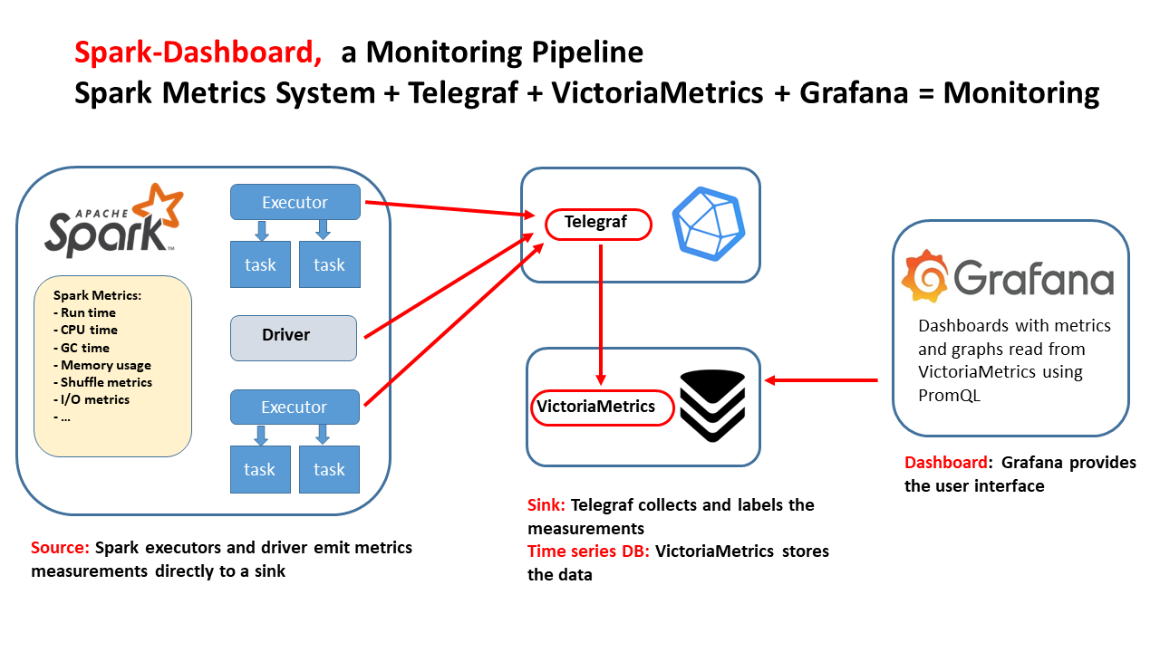
• Spark-Dashboard: Use this to monitor Spark jobs and visualize key performance metrics.

Additional tools for Performance Measurement include:

• Flame Graphs for Spark and Grafana Pyroscope with Spark
• Tools for OS performance monitoring

Demos

These quick demos and tutorials will show you how to use the tools in this Spark Performance Lab. You can follow along and get the same results on your own, which will help you start learning and exploring.

• SparkMeasure - metrics collection
•  Watch sparkMeasure's getting started demo and tutorial
• TPCDS_PySpark - workload generator
•  Watch TPCDS-PySpark demo and tutorial
• Spark-Dashboard - real-time dashboards
• Watch Spark-Dashboard demo and tutorial

Figure 1: The graph illustrates the dynamic task allocation in a Spark application during a TPCDS 10TB benchmark on a YARN cluster with 256 cores. It showcases the variability in the number of active tasks over time, highlighting instances of execution "long tails" and straggler tasks, as seen in the periodic spikes and troughs.

How to Make the Best of Spark Metrics System

Understanding and utilizing Spark's metrics system is crucial for optimization:

• Importance of Metrics: Metrics provide insights beyond simple timing, revealing details about task execution, resource utilization, and bottlenecks.
  
  
• Execution Time is Not Enough: Measuring the execution time of a job (how long it took to run it), is useful, but it doesn’t show the whole picture. Say the job ran in 10 seconds. It's crucial to understand why it took 10 seconds instead of 100 seconds or just 1 second. What was slowing things down? Was it the CPU, data input/output, or something else, like data shuffling? This helps us identify the root causes of performance issues.
  
  
• Key Metrics to Collect:
• Executor Run Time: Total time executors spend processing tasks.
• Executor CPU Time: Direct CPU time consumed by tasks.
• JVM GC Time: Time spent in garbage collection, affecting performance.
• Shuffle and I/O Metrics: Critical for understanding data movement and disk interactions.
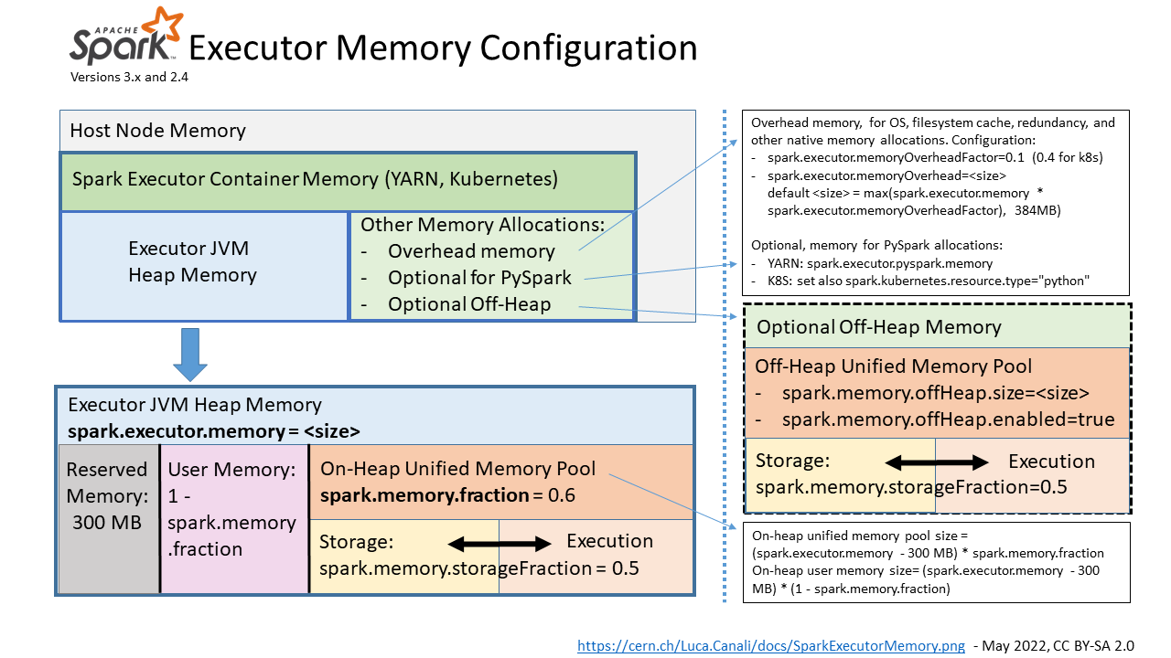
• Memory Metrics: Key for performance and troubleshooting Out Of Memory errors.
  
  
• Metrics Analysis, what to look for:
• Look for bottlenecks: are there resources that are the bottleneck? Are the jobs running mostly on CPU or waiting for I/O or spending a lot of time on Garbage Collection?
• USE method: Utilization Saturation and Errors (USE) Method is a methodology for analyzing the performance of any system. 
• The tools described here can help you to measure and understand Utilization and Saturation.
• Can your job use a significant fraction of the available CPU cores? 
• Examine the measurement of  the actual number of active tasks vs. time.
• Figure 1 shows the number of active tasks measured while running TPCDS 10TB on a YARN cluster, with 256 cores allocated. The graph shows spikes and troughs.
• Understand the root causes of the troughs using metrics and monitoring data. The reasons can be many: resource allocation, partition skew, straggler tasks, stage boundaries, etc.
• Which tool should I use?
• Start with using the Spark Web UI
• Instrument your jobs with sparkMesure. This is recommended early in the application development, testing, and for Continuous Integration (CI) pipelines.
• Observe your Spark application execution profile with Spark-Dashboard.
• Use available tools with OS metrics too. See also Spark-Dashboard extended instrumentation: it collects and visualizes OS metrics (from cgroup statistics) like network stats, etc
• Drill down:
• An example of Spark metrics analysis for TPCDS run at scale 10 TB

• Documentation: 
• For those interested in delving deeper into Spark instrumentation and metrics, the Spark documentation offers a comprehensive guide.
• SparkMeasure: This tool captures metrics directly from Spark’s instrumentation via the Listener Bus. For a detailed understanding of how it operates, refer to the SparkMeasure architecture. It specifically gathers data from Spark's Task Metrics System, which you can explore further here.
• Spark-Dashboard: This application aggregates metrics that Spark exposes through the Dropwizard metrics library (see Spark-Dashboard architecture). A complete list of the metrics can be found here.

Figure 2: This technical drawing outlines the integrated monitoring pipeline for Apache Spark implemented by Spark-Dashboard using open-source components. The flow of the diagram illustrates the Spark metrics source and the components used to store and visualize the metrics.

Lessons Learned and Conclusions

From setting up and running a Spark Performance Lab, here are some key takeaways:

• Collect, analyze and visualize metrics: Go beyond just measuring jobs' execution times to troubleshoot and fine-tune Spark performance effectively.
• Use the Right Tools: Familiarize yourself with tools for performance measurement and monitoring.
• Start Small, Scale Up: Begin with smaller datasets and configurations, then gradually scale to test larger, more complex scenarios.
• Tuning is an Iterative Process: Experiment with different configurations, parallelism levels, and data partitioning strategies to find the best setup for your workload.

Establishing a Spark Performance Lab is a fundamental step for any data engineer aiming to master Spark's performance aspects. By integrating tools like Web UI, TPCDS_PySpark, sparkMeasure, and Spark-Dashboard, developers and data engineers can gain unprecedented insights into Spark operations and optimizations. 

Explore this lab setup to turn theory into expertise in managing and optimizing Apache Spark. Learn by doing and experimentation!

Acknowledgements: A special acknowledgment goes out to the teams behind the CERN data analytics, monitoring, and web notebook services, as well as the dedicated members of the ATLAS database group.

Resources

To get started with the tools mentioned in this blog:

• TPCDS_PySpark
• SparkMeasure
• Spark-Dashboard and Dashboard Notes
• Flame Graphs for Spark and Grafana Pyroscope with Spark
• Tools for OS performance monitoring

Apache Spark 3.0 Memory Monitoring Improvements

TLDR; Apache Spark 3.0 comes with many improvements, including new features for memory monitoring. This can help you troubleshooting memory usage and optimizing the memory configuration of your Spark jobs for better performance and stability, see SPARK-23429 and SPARK-27189.

The problem with memory

Memory is key for the performance and stability of Spark jobs. If you don't allocate enough memory for your Spark executors you are more likely to run into the much dreaded Java OOM (out of memory) errors or substantially degrade your jobs' performance. Memory is needed by Spark to execute efficiently Dataframe/RDD operations, and for improving the performance of algorithms that would otherwise have to swap to disk in their processing (e.g. shuffle operations), moreover, it can be used for caching data, reducing I/O. This is all good in theory, but in practice how do you know how much memory you need?

A basic solution

One first basic approach to memory sizing for Spark jobs, is to start by giving the executors ample amounts of memory, provided your systems has enough resources. For example, by setting the spark.executor.memory configuration parameter to several GBs. Note, in local mode you would set sprk.driver.memory instead. You can further tune the configuration by trial-and-error, by reducing and increasing memory with each test and observe the results. This approach may give good results quickly, but it is not a very solid approach to the problem.

A more structured approach to memory usage troubleshooting and to sizing memory for Spark jobs is to use monitoring data to understand how much memory is used by the Spark application, which jobs request more memory, and which memory areas are used, finally linking this back to the application details and in the context of other resources utilization (for example, CPU usage).

This approach helps with drilling down on issues of OOM, and also to be more precise in allocating memory for Spark applications, aiming at using just enough memory as needed, without wasting memory that can be a scarce shared resource in some systems. It is still an experimental and iterative process, but more informed than the basic trial-and-error solution.

How memory is allocated and used by Spark

Configuration of executor memory

The main configuration parameter used to request the allocation of executor memory is spark.executor.memory.Spark running on YARN, Kubernetes or Mesos, adds to that a memory overhead  to cover for additional memory usage (OS, redundancy, filesystem cache, off-heap allocations, etc), which is calculated as memory_overhead_factor * spark.executor.memory  (with a minimum of 384 MB). The overhead factor is 0.1 (10%), it can be configured when running on Kubernetes (only) using spark.kubernetes.memoryOverheadFactor.

When using PySpark additional memory can be allocated using spark.executor.pyspark.memory. 

Additional memory for off-heap allocation is configured using spark.memory.offHeap.size=<size> and spark.memory.offHeap.enabled=true. This works on YARN, for K8S, see SPARK-32661.  

Note also parameters for driver memory allocation: spark.driver.memory and spark.driver.memoryOverhead. 

Note: this covers recent versions of Spark at the time of this writing, notably Spark 3.0 and 2.4. See also Spark documentation.

  

Figure 1: Pictorial representation of the memory areas allocated and used by Spark executors and the main parameters for their configuration. 

• Image in png format: SparkExecutorMemory.png
• Image source, in powerpoint format: SparkExecutorMemory.pptx

  

Spark unified memory pool

Spark tasks allocate memory for execution and storage from the JVM heap of the executors using a unified memory pool managed by the Spark memory management system. Unified memory occupies by default 60% of the JVM heap: 0.6 * (spark.executor.memory - 300 MB). The factor 0.6 (60%) is the default value of the configuration parameter spark.memory.fraction. 300MB is a hard-coded value of "reserved memory". The rest of the memory is used for user data structures, internal metadata in Spark, and safeguarding against OOM errors. 

Spark manages execution and storage memory requests using the unified memory pool. When little execution memory is used, storage can acquire most of the available memory, and vice versa. Additional structure in the working of the storage and execution memory is exposed with the configuration parameter spark.memory.storageFraction (default is 0.5), which guarantees that the stored blocks will not be evicted from the unified memory by execution below the specified threshold.

The unified memory pool can optionally be allocated using off-heap memory, the relevant configuration parameters are: spark.memory.offHeap.size and spark.memory.offHeap.enabled. 

  

Opportunities for memory configuration settings

The first key configuration to get right is spark.executor.memory. Monitoring data (see the following paragraphs) can help you understand if you need to increase the memory allocated to Spark executors and or if you are already allocating plenty of memory and can consider reducing the memory footprint.

There are other memory-related configuration parameters that may need some adjustments for specific workloads: this can be analyzed and tested using memory monitoring data.

In particular, increasing spark.memory.fraction (default is 0.6) may be useful when deploying large Java heap, as there is a chance that you will not need to set aside 40% of the JVM heap for user memory. With similar reasoning, when using large Java heap allocation, manually setting spark.executor.memoryOverhead to a value lower than the default (0.1 * spark.executor.memory) can be tested.

  

Memory monitoring improvements in Spark 3.0

Two notable improvements in Spark 3.0 for memory monitoring are:

• SPARK-23429: Add executor memory metrics to heartbeat and expose in executors REST API
• see also the umbrella ticket SPARK-23206: Additional Memory Tuning Metrics
• SPARK-27189: Add Executor metrics and memory usage instrumentation to the metrics system

When troubleshooting memory usage it is important to investigate how much memory was used as the workload progresses and measure peak values of memory usage. Peak values are particularly important, as this is where you get possible slow downs or even OOM errors. Spark 3.0 instrumentation adds monitoring data on the amount of memory used, drilling down on unified memory, and memory used by Python (when using PySpark). This is implemented using a new set of metrics called "executor metrics", and can be helpful for memory sizing and troubleshooting performance. 

    

Measuring memory usage and peak values using the REST API

An example of the data you can get from the REST API in Spark 3.0:

WebUI URL + /api/v1/applications/<application_id>/executors

Here below you can find a snippet of the peak executor memory metrics, sampled on a snapshot and limited to one of the executors used for testing:

"peakMemoryMetrics" : {
    "JVMHeapMemory" : 29487812552,
    "JVMOffHeapMemory" : 149957200,
    "OnHeapExecutionMemory" : 12458956272,
    "OffHeapExecutionMemory" : 0,
    "OnHeapStorageMemory" : 83578970,
    "OffHeapStorageMemory" : 0,
    "OnHeapUnifiedMemory" : 12540212490,
    "OffHeapUnifiedMemory" : 0,
    "DirectPoolMemory" : 66809076,
    "MappedPoolMemory" : 0,
    "ProcessTreeJVMVMemory" : 38084534272,
    "ProcessTreeJVMRSSMemory" : 36998328320,
    "ProcessTreePythonVMemory" : 0,
    "ProcessTreePythonRSSMemory" : 0,
    "ProcessTreeOtherVMemory" : 0,
    "ProcessTreeOtherRSSMemory" : 0,
    "MinorGCCount" : 561,
    "MinorGCTime" : 49918,
    "MajorGCCount" : 0,
    "MajorGCTime" : 0
  },

Notes:

• Procfs metrics (SPARK-24958) provide a view on the process usage from "the OS point of observation".
• Notably, procfs metrics provide a way to measure memory usage by Python, when using PySpark and in general other processes that may be spawned by Spark tasks.
• Profs metrics are gathered conditionally:
• if the /proc filesystem exists
• if spark.executor.processTreeMetrics.enabled=true
• The optional configuration spark.executor.metrics.pollingInterval allows to gather executor metrics at high frequency, see doc.
• Additional improvements of the memory instrumentation via REST API (targeting Spark 3.1) are in "SPARK-23431 Expose the new executor memory metrics at the stage level".
  

  

Improvements to the Spark metrics system and Spark performance dashboard

The Spark metrics system based on the Dropwizard metrics library provides the data source to build a Spark performance dashboard. A dashboard naturally leads to time series visualization of Spark performance and workload metrics. Spark 3.0 instrumentation (SPARK-27189) hooks to the executor metrics data source and makes available the time series data with the evolution of memory usage. 

Some of the advantages of collecting metrics values and visualizing them with Grafana are:

• The possibility to see the evolution of the metrics values in real time and to compare them with other key metrics of the workload. 
• Metrics can be examined as aggregated values or drilled down at the executor level. This allows you to understand if there are outliers or stragglers.
• It is possible to study the evolution of the metrics values with time and understand which part of the workload has generated certain spikes in a given metric, for example. It is also possible to annotate the dashboard graphs, as explained at this link, with details of query id, job id, and stage id.

Here are a few examples of dashboard graphs related to memory usage:

Figure 2: Graphs of memory-related  metrics collected and visualized using a Spark performance dashboard. Metrics reported in the figure are: Java heap memory, RSS memory, Execution memory, and Storage memory. The Grafana dashboard allows us to drill down on the metrics values per executor. These types of plots can be used to study the time evolution of key metrics.

  

What if you are using Spark 2.x?

Some monitoring features related to memory usage are already available in Spark 2.x and still useful in Spark 3.0:

• Task metrics are available in the REST API and in the dropwizard-based metrics and provide information:
• Garbage Collection time: when garbage collection takes a significant amount of time typically you want to investigate for the need for allocating more memory (or reducing memory usage).
• Shuffle-related metrics: memory can prevent some shuffle operations with I/O to storage and be beneficial for performance.
• Task peak execution memory metric.
• The WebUI reports storage memory usage per executor.
• Spark dropwizard-based metrics system provides a JVM source with memory-related utilization metrics.

  

Lab configuration:

When experimenting and trying to get a grasp for the many parameters related to memory and monitoring, I found it useful to set up a small test workload. Some notes on the setup I used:

• Tested using Spark 3.0 on YARN and Kubernetes.  
• Spark performance dashboard: configuration and installation instruction for the Spark dashboard at this link.  
• Workload generator: TPCDS benchmark for Spark, with a small modification to run on Spark 3.0.  Example:

bin/spark-shell --master yarn --num-executors 16 --executor-cores 8 \

--driver-memory 4g --executor-memory 32g \

--jars /home/luca/spark-sql-perf/target/scala-2.12/spark-sql-perf_2.12-0.5.1-SNAPSHOT.jar \

--conf spark.eventLog.enabled=false \

--conf spark.sql.shuffle.partitions=512 \

--conf spark.sql.autoBroadcastJoinThreshold=100000000 \

--conf spark.executor.processTreeMetrics.enabled=true

  

  

import com.databricks.spark.sql.perf.tpcds.TPCDSTables

val tables = new TPCDSTables(spark.sqlContext, "/home/luca/tpcds-kit/tools","1500")

tables.createTemporaryTables("/project/spark/TPCDS/tpcds_1500_parquet_1.10.1", "parquet")

val tpcds = new com.databricks.spark.sql.perf.tpcds.TPCDS(spark.sqlContext)

val experiment = tpcds.runExperiment(tpcds.tpcds2_4Queries)

  

Limitations and caveats

• Spark metrics and instrumentation are still an area in active development. There is room for improvement both in their implementation and documentation. I found that some of the metrics may be difficult to understand or may present what looks like strange behaviors in some circumstances. In general, more testing and sharing experience between Spark users may be highly beneficial for further improving Spark instrumentation.
• The tools and methods discussed here are based on metrics, they are reactive by nature, and suitable for troubleshooting and iterative experimentation.
• This post is centered on  describing Spark 3.0 new features for memory monitoring and how you can experiment with them. A key piece left for future work is to show some real-world examples of troubleshooting using memory metrics and instrumentation.
• For the scope of this post, we assume that the workload to troubleshoot is a black box and that we just want to try to optimize the memory allocation  and use. This post does not cover techniques to improve the memory footprint of Spark jobs, however, they are very important for correctly using Spark. Examples of techniques that are useful in this area are: implementing the correct partitioning scheme for the data and operations, reducing partition skew, using the appropriate join mechanisms, streamlining caching, and many others, covered elsewhere. 

  

References

Talks:

• Metrics-Driven Tuning of Apache Spark at Scale, Spark Summit 2018.
• Performance Troubleshooting Using Apache Spark Metrics, Spark Summit 2019
• Tuning Apache Spark for Large-Scale Workloads, Spark summit 2017
• Deep Dive: Apache Spark Memory Management, Spark Summit 2016.
• Understanding Memory Management In Spark For Fun And Profit, Spark Summit 2016.

Spark documentation and blogs:

• Monitoring guide: REST API, Executor Task Metrics. Executor Metrics, Spark Metrics System
• Tuning guide: Memory Management Overview
• Apache Spark and off-heap memory
• Apache Spark Memory Management: Deep Dive
• A Performance Dashboard for Apache Spark

JIRAs:  SPARK-23206, SPARK-23429 and SPARK-27189 contain most of the details of the improvements in Apache Spark discussed here.

Spark code: Spark Memory Manager, Unified memory

  

Conclusions and acknowledgments

It is important to correctly size memory configurations for Spark applications. This improves performance, stability, and resource utilization in multi-tenant environments. Spark 3.0 has important improvements to memory monitoring instrumentation. The analysis of peak memory usage, and of memory use broken down by area and plotted as a function of time, provide important insights for troubleshooting OOM errors and for Spark job memory sizing.   

Many thanks to the Apache Spark community, and in particular the committers and reviewers who have helped with the improvements in SPARK-27189.

This work has been developed in the context of the data analytics services at CERN, many thanks to my colleagues for help and suggestions.  

  

Extended Stack Profiling - Ideas, Tools and Comments

Topic: This post provides a short summary and pointers to previous work on Extended Stack Profiling for troubleshooting and performance investigations.

Understanding the workload is an important part of troubleshooting activities. We seek answers to questions like: what is the system doing, where is the time spent, which code paths are most used, what are the wait events, etc. Sometimes the relevant diagnostic data is easy to find, other times we need to dig deeper. Stack profiling and flame graph visualizations are very useful techniques for advanced troubleshooting. In particular in the Linux environment stack traces gathered with perf provide a quick and powerful window into CPU-bound workloads, as detailed in the work of Brendan Gregg.

Extended Stack Profiling techniques stem from the experience of using on-CPU stack profiles and flame graphs. The basic idea is to pull together stack traces with OS- and application-specific metrics. This has the advantage of exposing the inner workings of the process under investigation, together with the context of its execution, such as its parent functions and the execution of kernel functions, when relevant. Application metrics that can also be added. Notably, when examining Oracle workloads, data from the wait event interface can be added as an additional dimension to the stack traces.

Examples of using extended stack tracing tools for troubleshooting and investigating Oracle workloads can be found in these blog articles: "Linux Kernel Stack Profiling and Flame Graphs Applied to Oracle Investigations", "Oracle Wait Events Investigated with Extended Stack Profiling and Flame Graphs" and in the presentation "Stack Traces & Flame Graphs for Oracle Troubleshooting".
Three tools and code examples complement the blog articles:

• KStackSampler: a tool written in shell script which gathers kernel stack profiling together and process status. 
• ORA_KStackProfiler: a simple kernel stack profiler written in C, extended with process status information and the option of sampling Oracle wait event information from SGA.
• Ptrace_Profiler: an extension of ORA_KStackProfiler with userspace stack sampling implemented using ptrace and libunwind.

Pros: techniques based on extended stack profiling allow to investigate Oracle workloads beyond what is available with the wait event interface. In particular when combined with flame graph visualization they provide insights into the inner workings of complex workloads, which in turns can be used to complement or extend what is available with Oracle instrumentation. The techniques are general and can be used or to troubleshoot many and diverse Linux workloads.

Cons: Limitations of the code discussed here are many and the tools have to to be considered as experimental. One of the main issues is the error that is intrinsic when pasting together different data sources, such as stack traces and process status, that are collected sequentially by the tools. This is particularly evident with the ptrace-based implementation for userspace stack traces which requires to stop the process for a relatively long time (can be 100s of milliseconds). The fact that data collection is based on sampling introduces another potential source of error. The sampling frequency has to be adapted to the workload: not too high to limit the overhead, not too low to avoid losing the details of rapidly varying workloads. Some other 'gotchas' come from the use of flame graphs, in particular it is worth reminding that the horizontal axis of those graphs does not represent the time evolution.

Ideas for future work: the tools can be extended by developing the interfaces to sample more data sources. For Oracle this could be adding more fields from V$SESSION (X$KSUSE) or other V$/X$ structures. More generally, probes can be developed for sampling and investigating a larger range of applications, similarly and extending the the work done for Oracle. Extension for multi-threaded processes would also make the tools more generic. A user interface to simplify the selection of the data sources and integration with flame graph visualization would also be beneficial.
Another area for improvement is with userspace stack tracing. It is currently implemented in Ptrace_Profiler by stopping the process while unwinding the stack, a simple method with a high overhead. There are better methods: for example with techniques for asynchronous stack unwinding that allow to stop the process for a much shorter time. This would reduce the footprint of the measurement and also allow for higher sampling frequency.
Additional work is also needed to better understand the reliability of the measurements and the errors incurred when sampling and pasting together (on-the-fly) the various data sources, as discussed above.

Credits and additional references: Brendan Gregg is the inventor of flame graphs and has published excellent material on this and other related topics of interest for troubleshooting performance. Tanel Poder has covered the topic of stack profiling and many others of interest in his blog. Additional and related investigations of Oracle internals can be found in the blog of Frits Hoogland and in the blog of Stefan Koehler.
Links to previous work: "Linux Kernel Stack Profiling and Flame Graphs Applied to Oracle Investigations", "Oracle Wait Events Investigated with Extended Stack Profiling and Flame Graphs", "Stack Traces & Flame Graphs for Oracle Troubleshooting", "Oracle Optimizer Investigated with Flame Graphs", "Flame Graphs for Oracle". Tools referenced in this post are available on Github and at this web page.

Diagnose High-Latency I/O Operations Using SystemTap

Topic: this post is about some simple tools and techniques that can be used to drill down high-latency I/O events using SystemTap probes.

The problem: Operations with high latency on a filesystem and/or a storage volume can sometimes be attributed to just a few disks 'misbehaving', possibly because they are suffering mechanical failures and/or are going to break completely in the near future.
I/Os of high latency on just a few disks can then appear as latency outliers when accessing volumes build on a large number of disks and overall affect the performance of the entire storage. I write this having in mind the example of a storage system built with (SATA) JBODs using Oracle ASM as volume manager/DB filesystem. However the main ideas and tools described in this post apply to many other volume managers and file systems, including HDFS.

The standard tools: One way to find that one or more disks are serving I/O requests with high latency is with the use of standard Linux tools such as iostat, sar or collectl. Typically you would use those tools to spot anomalous values of average service time, average wait time and also of queue size.
A structured approach on how to do this is described in Brendan Gregg's USE method and the tools that can be used in Linux to implement it.

SystemTap scripts: In this post we focus on a technique and a couple of simple scripts that can be used to identify disks serving I/O with high latency using SystemTap probes to investigate I/O latency of the block devices.
The script blockio_latency_outliers_per_device.stp provides a measurement of some basics latency statistics for block device, including number of I/Os, average and maximum latency. The script also provides details of all the I/O where the latency is above a certain programmable threshold (the default threshold is set at 500 microseconds).
An example of its use (edited output for clarity) is here below. Note the latency warning message and overall the very large maximum value measured for the latency of the /dev/sdy block device:

[root@myhost] # stap -v blockio_latency_outliers_per_device.stp 10

Measuring block I/O latency and statistics
A warning will be printed for I/Os with latency higher than 500000 microseconds
Statistics will be printed every 10 seconds. Press CTRL-C to stop

...

latency warning, >500000 microsec: device=sdy, sector=166891231, latency=714984
latency warning, >500000 microsec: device=sdy, sector=165679327, latency=582708
latency warning, >500000 microsec: device=sdy, sector=167102975, latency=1162550

....

I/O latency basic statistics per device, measurement time: 10 seconds
Latency measured in microseconds

Disk name          Num I/Os    Min latency    Avg latency    Max latency

....

sdu                     219            106           6217          27117
sdz                     200            123           5995          27205
sdq                     211             71           6553          31120
sdh                     256            103           6643          22663
sds                     224            101           6610          29743
sdm                     238             92           7550          35571
sde                     243             90           8652          52029
sdt                     200            105           5997          25180
sdk                     200             94           5696          35057
sdi                     206             99           7849          30636
sdg                     269             74           6746          36746
sdy                     197            102          98298        1167977
sdr                     200             89           6559          27873
sdl                     200            140           8789          31996
sdw                     210             99           7009          37118
sdd                     217             94           7440          56071
sdn                     205             99           6628          41339
....

When candidate disks for high latency have been identified, the second step is to further drill down using the script blockio_rq_issue_filter_latencyhistogram.stp. This script gathers and displays I/O latency histograms for a subset of block devices that can be specified using filters in the script header. The default filters are:

# SystemTap variables used to define filters, edit as needed
global IO_size = 8192    # this will be used as a filter for the I/O request size
                         # the value 8192 targets 8KB operations for Oracle single-block I/O
                         # use the value -1 to disable this filter
global IO_operation = 0  # this will be used as a filter: only read operations
                         # a value of 0 considers only read operations (the value 1 is for write)
                         # use the value -1 to disable this filter
global IO_devmaj = -1    # this will be used as a filter: device major number (-1 means no filter)
                         # example: use the value 253 for device mapper block devices
global IO_devmin = -1    # device minor number (or -1 if no filter)

You can use  blockio_rq_issue_filter_latencyhistogram.stp to drill down on the latency histogram for those disks that have shown high latency I/O and also compare them with "good" disks. In the example above the candidate "trouble disk" is /dev/sdy with major number 65 and minor 128 (you can major and minor device numbers for "sdy" simply using ls -l /dev/sdy).
Example:

stap -v blockio_rq_issue_filter_latencyhistogram.stp 10

Block I/O latency histograms from kernel trace points
Filters:
    IO_size = 8192
    IO_operation = 0 (0=read, 1=write, -1=disable filter)
    IO_devmaj = 65 (-1=disable filter)
    IO_devmin = 128 (-1=disable filter)

lock I/O latency histogram, measurement time: 10 seconds, I/O count: 199
Value = latency bucket (microseconds), count=I/O operations in 10 seconds
  value |-------------------------------------------------- count
     16 |                                                    0
     32 |                                                    0
     64 |@                                                   2
    128 |@@@@@@@                                            14
    256 |@@                                                  4
    512 |@                                                   2
   1024 |@@@                                                 7
   2048 |@@@@@@@@@                                          19
   4096 |@@@@@@@@@@@@@@@@@@                                 37
   8192 |@@@@@@@@@@@@@@@@@@@@@@@@@@@@@                      59
  16384 |@@@@@@@                                            14
  32768 |                                                    0
  65536 |@@@@@          HIGH                                10
 131072 |@@@@@          LATENCY                             11
 262144 |@@@@@          I/O                                 10
 524288 |@@@            OPERATIONS                           6
1048576 |@@                                                  4
2097152 |                                                    0

Note the presence of several I/O operations at high latency together with more normal I/O latecy, for example I/Os served from SATA disks at around 8 ms and also I/O served from the controller cache at sub-millisecond latency.
For comparison here below is the latency histogram measured on another disk while the same workload was running. We can see that in this case high latency points found in the previous example are no more present. Most of the I/O operations are around 8 ms latency and some operations served from cache at sub-millisecond latency. The I/O reported for the /dev/sdy disks with latency of 64 ms and above are not present in this case.

stap -v blockio_rq_issue_filter_latencyhistogram.stp 10

Block I/O latency histograms from kernel trace points
Filters:
    IO_size = 8192
    IO_operation = 0 (0=read, 1=write, -1=disable filter)
    IO_devmaj = 65 (-1=disable filter)
    IO_devmin = 48 (-1=disable filter)


Block I/O latency histogram, measurement time: 10 seconds, I/O count: 196
Value = latency bucket (microseconds), count=I/O operations in 10 seconds
value |-------------------------------------------------- count
   32 |                                                    0
   64 |                                                    0
  128 |@@@@@@@@@                                          19
  256 |@@@@@@@@                                           16
  512 |                                                    1
 1024 |@@@@                                                9
 2048 |@@@@@@@@@@@@@@                                     28
 4096 |@@@@@@@@@@@@@@@@@@@@@@@@@@@@                       56
 8192 |@@@@@@@@@@@@@@@@@@@@@@@@                           49
16384 |@@@@@@@@@                                          18
32768 |                                                    0
65536 |                                                    0

The tests reported here have been performed on a old system running RHEL 5 (kernel 2.6.18-371)  and SystemTap v. 1.8, however the scripts have also been tested on OL and CentOS 7.1 (kernel 3.10.0-229) and SystemTap 2.8. If you are using SystemTap 2.6 or above you can use the scripts blockio_rq_issue_latencyhistogram_new.stp and blockio_rq_issue_filter_latencyhistogram_new.stp instead.

Conclusion: In this post we have shown a simple technique to diagnose I/O latency outliers and in particular on how to drill down on I/Os served at high latency because of one or more misbehaving disk in the storage volume/filesystem. The investigation has been done using SystemTap scripts used first to discover which disks were serving some of their I/O s with high latency and then drilling down on specific devices with the use of latency histograms. The fact of identifying and later replacing the badly performing disks can be beneficial for the performance of the entire storage systems.

Download: The tools discussed in this post can be downloaded from this webpage and from Github.

Acknowledgements and additional links: Brendan Gregg has published an extensive set of articles and tools on performance tuning, including storage latency investigations.
For more information and examples on how to use SystemTap see the SystemTap wiki
Additional tools for Oracle ASM I/O investigations also see Bertrand Drouvot's asm_metrics.pl
Kevin Closson's SLOB was used as workload generator for the examples discussed here.
Additional links on tools and techniques on Oracle I/O troubleshooting in this blog: Heat Map Visualization of I/O Latency with SystemTap and PyLatencyMap, Event Histogram Metric and Oracle 12c and Life of an Oracle I/O: Tracing Logical and Physical I/O with Systemtap